

Introduction
Species distribution models (SDMs) are among the statistical models that are used to predict the potential distribution of a species based on environmental factors such as temperature, precipitation, and topography. These models are utilized to identify regions that are appropriate for a specific species to inhabit. This can aid in informing conservation and management efforts [1-2]. There are several different types of SDMs, each with their own strengths and weaknesses. One of the most widely used types of SDMs is the bioclimatic envelope model. This model uses a combination of climate data and species occurrence data to predict the potential distribution of a species. The model is based on the idea that a species distribution is limited by the environmental conditions that it can tolerate. For instance, a species that lives in a desert would have a different bioclimatic envelope than a species that lives in a tropical rainforest [3-5]. Another type of SDM is the machine learning-based model. These models use a combination of environmental variables and species occurrence data to predict the possible distribution of a species. They use algorithms, such as random forests and support vector machines, that can handle large and complex datasets. These models are becoming increasingly popular because they can make predictions with high accuracy and can also determine the most important site factors that are affecting the species distribution [6-10].
An important part of SDM is to use quality data. This can include both occurrence data of species and the environmental variable data. Occurrence data can be collected through a variety of methods such as surveys, online databases, or museum/herbarium records. These data are used to train and validate the models. Environmental variable data are also important, as the models use this data to make predictions about the distribution of a species. These data can be acquired from a variety of sources, such as remote sensing and climate prediction models [11]. Once the models are trained and validated, they can be used to make predictions about the potential distribution of a species. The predictions generated by these models can be utilized to identify regions that are appropriate for the distribution of a certain species. This information can assist in guiding conservation and management initiatives. For instance, SDMs can be employed to identify regions that are crucial for the preservation of a particular species, such as areas that are at high risk of habitat loss or fragmentation.
With the advances in machine learning, many new algorithms have been developed. In this way, it has become more powerful and effective in making predictions. Although the existence of many methods complicates the process, researchers mostly choose the most appropriate method in line with their hypotheses and overcome this difficulty. In recent studies, methods such as Ecological Niche Factor Analysis (ENFA), (MaxEnt), Random Forest, Generalized Additive Model (GAM), Classification and Regression Tree (CART), Genetic Algorithm for Rule Set Production (GARP), DOMAIN, and Maximum Entropy are preferred more frequently [12-14]. In fact, the changing scientific perspective paves the way for the use of different algorithms in SDMs. Deep Learning is one of these algorithms [15]. However, once the method is chosen, all the problems do not disappear. The solution to one problem brings with it another problem. George Bernard Shaw, who is an Irish playwright, polemicist, political activist, and critic said the best words to express this process: “Science can never solve one problem without raising ten more problems” [16].
After choosing the suitable method, the first thing to do is to fit the occurrence data and environmental layers in accordance with the method. However, determining the resolution of the layers is an important criterion when choosing environmental variables. Resolution preference is of great importance especially for species distribution models on climate change. Because determining the distribution of target species in current and future climatic conditions reveals ecologically important results.
There are many databases from which climate data can be downloaded. CHELSA and WORLDCLIM are the most common and most preferred among them. Climate data in different resolutions can be downloaded from databases. When downloading the climate data, if the way of obtaining it via the website is preferred, the data is downloaded on a world scale. However, open-source types of software such as R and Python also offer the opportunity to download climate data only within a certain area. For instance, the WORLDCLIM database contains bioclimatic data for both the current and the future with resolutions of 30 arc seconds (~1 km), 2.5 arc minutes (~4.5 km), 5 arc minutes (~9 km), and 10 arc minutes (~18.5 km). Studies conducted in large areas using high-resolution bioclimatic variables (30 arc seconds) bring some difficulties. Handling big data is one of these challenges. Here, we are faced with a new question: “What should be the size of the area we will studying on?”. Two principal approaches can be taken into consideration while searching for an answer to this question. First of all, it may be an advantage to prefer the study area as large as possible in climate studies. Because preferring a large area in climate studies provides an advantage to detect the movement of a species and to determine how changes occur in the potential suitable areas of the related species. The second is the real-life applicability of the obtained potential suitability maps. In other words, it is the ability of the maps obtained to be included in the plans. In areas/countries with high topographical diversity, decision-makers carry out their planning in basins and sub-basins drawn according to ecological properties. Because these units and decision-makers are independent, it is more realistic and practical for them to make plans in the areas they are responsible for. However, it is also possible to make large-scale plans for a single target species. So much so that the basins and sub-basins are large enough in scale. Therefore, based on the information given, it is possible to work with environmental layers with different resolutions depending on the size of the study area. This result appears to be subjective at first glance. However, the resolution preference of bioclimatic variables can be made objectively. From this point of view, it is aimed to determine the effects of resolution preference on model performance by downloading the presence data of two different invasive plant species (Ambrosia artemisiifolia and Ailanthus altissima) from the Global Biodiversity Information Facility (GBIF) database in the present study. The potential distributions of these species were modeled with bioclimatic variables obtained at 3 different resolutions. An objective approach to resolution preference is presented by comparing the performances of the models obtained.
Materials and Methods
Study Area and Occurrence Data
In the present study, since modeling was performed for three different resolutions, it was more correct to prefer a wide area. Especially considering the 10 arc minutes resolution, it was thought that selecting a wide area would yield more reasonable results. Since there is a wide area, it has become a necessity to prefer species with a wide distribution. Because if a species with a local distribution was selected, the evaluation of bioclimatic variables would be far from being objective due to its microclimatic properties. That is why Ambrosia artemisiifolia (ragweed) and Ailanthus altissima (tree of heaven) which have wide distributions in Europe were selected as target species. Both of these species are considered invasive plants. While invasive species affect human health, they are widely distributed and quickly adapt to different habitat factors, they also show suppressive properties on other plant species. Therefore, both the effect of the resolution was investigated in the study, and useful information about the distribution of two important invasive plant species was presented. The occurrence data of the species were downloaded from the GBIF database [17-21].
Bioclimatic Variables
In traditional modeling studies where bioclimatic variables [22] are used, variable selection processes are mostly used, in which methods such as correlation analysis and principal component analysis are preferred [2, 13-14]. However, when the variable selection process was applied, different bioclimatic variables could be selected for a species in three models (for three different resolutions). This choice would have deprived the process of an objective evaluation. Therefore, the multi-collinearity problem has been ignored.
Predictive Modeling
MaxEnt was performed to model species distributions. MaxEnt is one of the most preferred methods in SDM in recent years. It only runs with present data and stands out with its features such as exhibiting good model performances with little data and producing models with high accuracy [23-25].
Evaluation of Model Performances
In order to compare the model performances, firstly, the occurrence data were transferred to the prediction maps and the predictive values corresponding to the points were determined. Then, the averages of the predictive values corresponding to the occurrences on the model maps of three different resolutions were compared.
As another performance evaluation method, 20% random data was chosen from the occurrences of both species, and this data was not included in the modeling. The predictive values of the model maps were categorized to represent suitable and unsuitable areas according to the 0.5 threshold value, and the percentage rates of the thresholded data corresponding to the randomly selected occurrence data were determined.
The last method used to evaluate model performances is the Area Under Curve (AUC) values of the models obtained for three different resolutions for each species.
Results and Discussion
In the present study, species distribution models were performed using bioclimatic variables with different resolutions for two invasive species. Statistically significant differences were found between the models obtained with different resolutions for both species.
Results for Ambrosia artemisiifolia (A. artemisiifolia)
The first species modeled in the study is A. artemisiifolia, an annual plant of the Asteraceae family that was first described by Carl Linnaeus in the 18th century. A. artemisiifolia, commonly known as common ragweed, is a harmful invasive weed that has a significant impact on agriculture. It is also a major source of highly allergenic pollen. This species is widely recognized as a problem, as demonstrated by the numerous international initiatives currently being undertaken by the European Commission, as well as the increasing number of publications dedicated to this topic [26-28]. This species has a large ecological tolerance range and, accordingly, a wide distribution. There are studies expressing that A. artemisiifolia is distributed in southern Europe [29], central and eastern Europe [30-32], north of the Black Sea, and Russia [33-34]. It even takes part in studies that reveal the existence of A. artemisiifolia in China and the United States [35-36]. One of the striking common points of these studies is the rapid spread of A. artemisiifolia [30]. This is due to its adaptability and raises two possible problems. So much so that these problems can be mentioned for many invasive species [37]. The first of the problems is that the rapid spread of A. artemisiifolia endangers the existence of many plant species. The other is that many people suffer from the allergic characteristics of this strain. For instance, one study found that 10% of the Croatian population had an allergic reaction to this species [31, 38].
In the present study, the Kruskal Wallis test was used to determine whether there is a difference between the predictive values of the potential distribution maps obtained for different resolutions. The Kruskal Wallis Test is a non-parametric method [39]. In order to decide which method should be preferred, the Kolmogorov-Smirnov normality test was performed using the predicted values. Test results showed that the data were not normally distributed (p<0.05).
Fig. 1.
Group averages of the predictive values obtained from the models made for different resolutions of the A. Artemisiifolia.
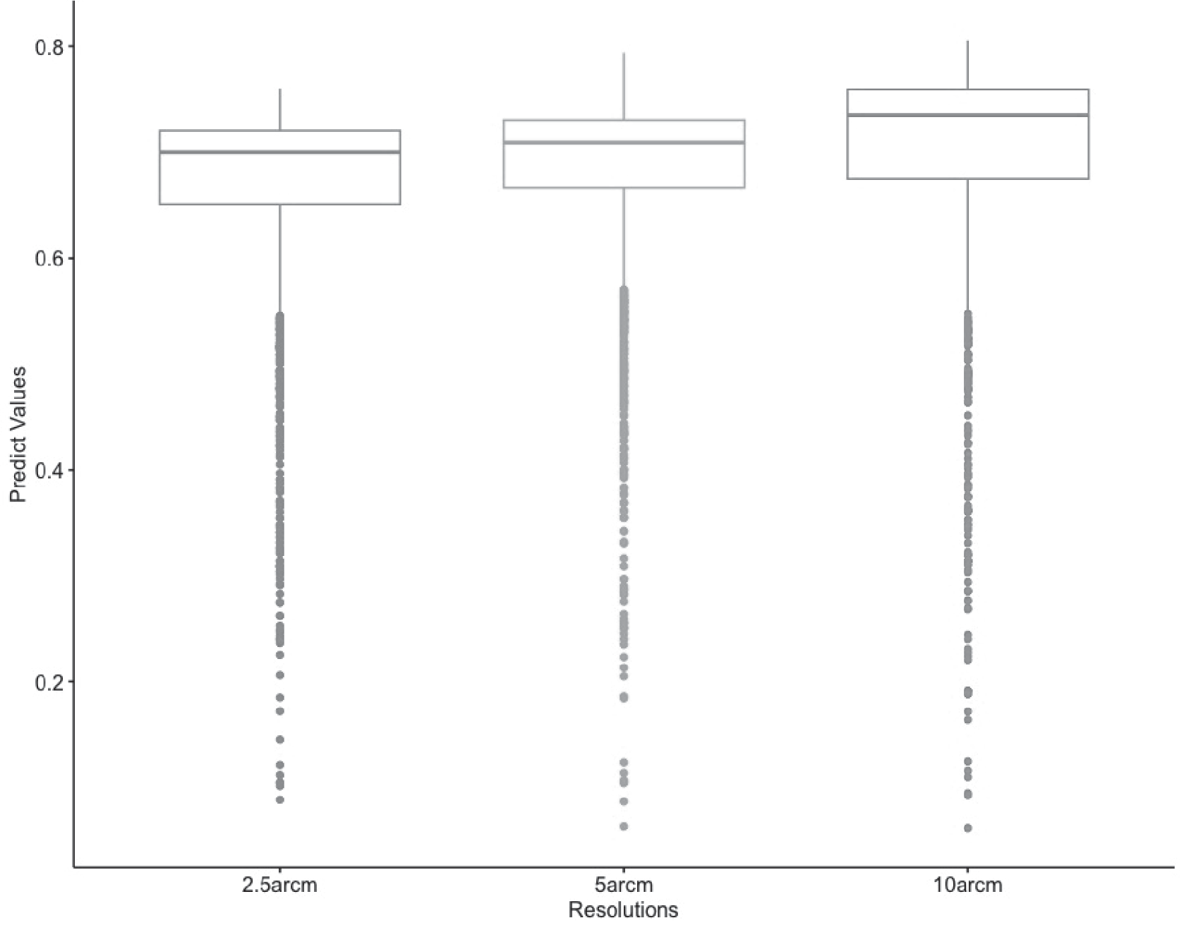
Kruskal Wallis rank sum test results revealed that there were significant differences between the modeling results obtained for A. artemisiifolia at different resolutions (p<0.05).
As depicted in Fig. 1, the Kruskal Wallis test results indicate that the variation in predicted values is a result of the model constructed using bioclimatic variables at a resolution of 10 arc minutes.
On the other hand, according to the MaxEnt models obtained in the study, it was determined that the factors affecting the distribution of the species were mostly heat-related factors (Bio_1, Bio_4, Bio_6) and precipitation of driest month (Bio_14). These results hint that potential areas may expand in the future.
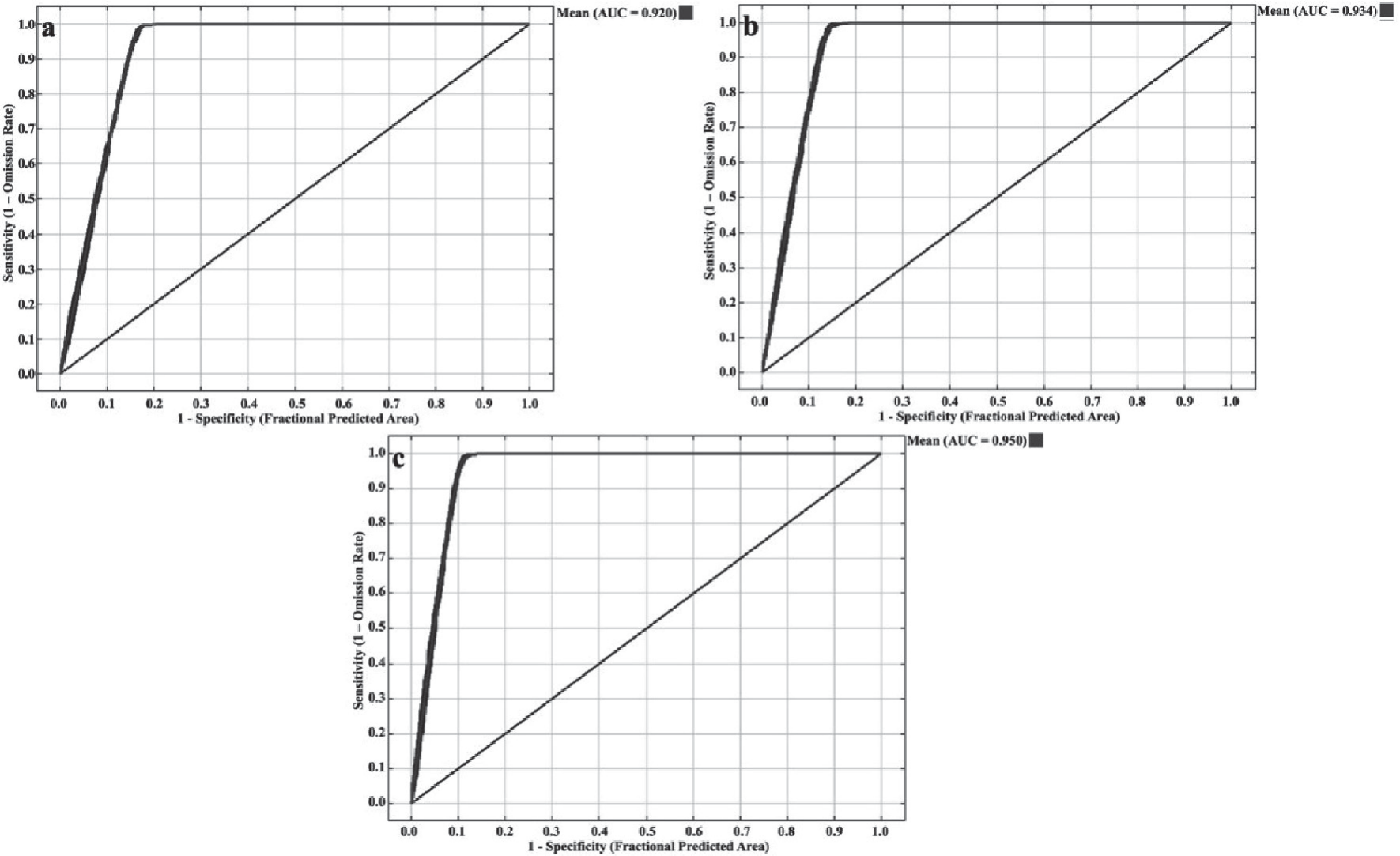
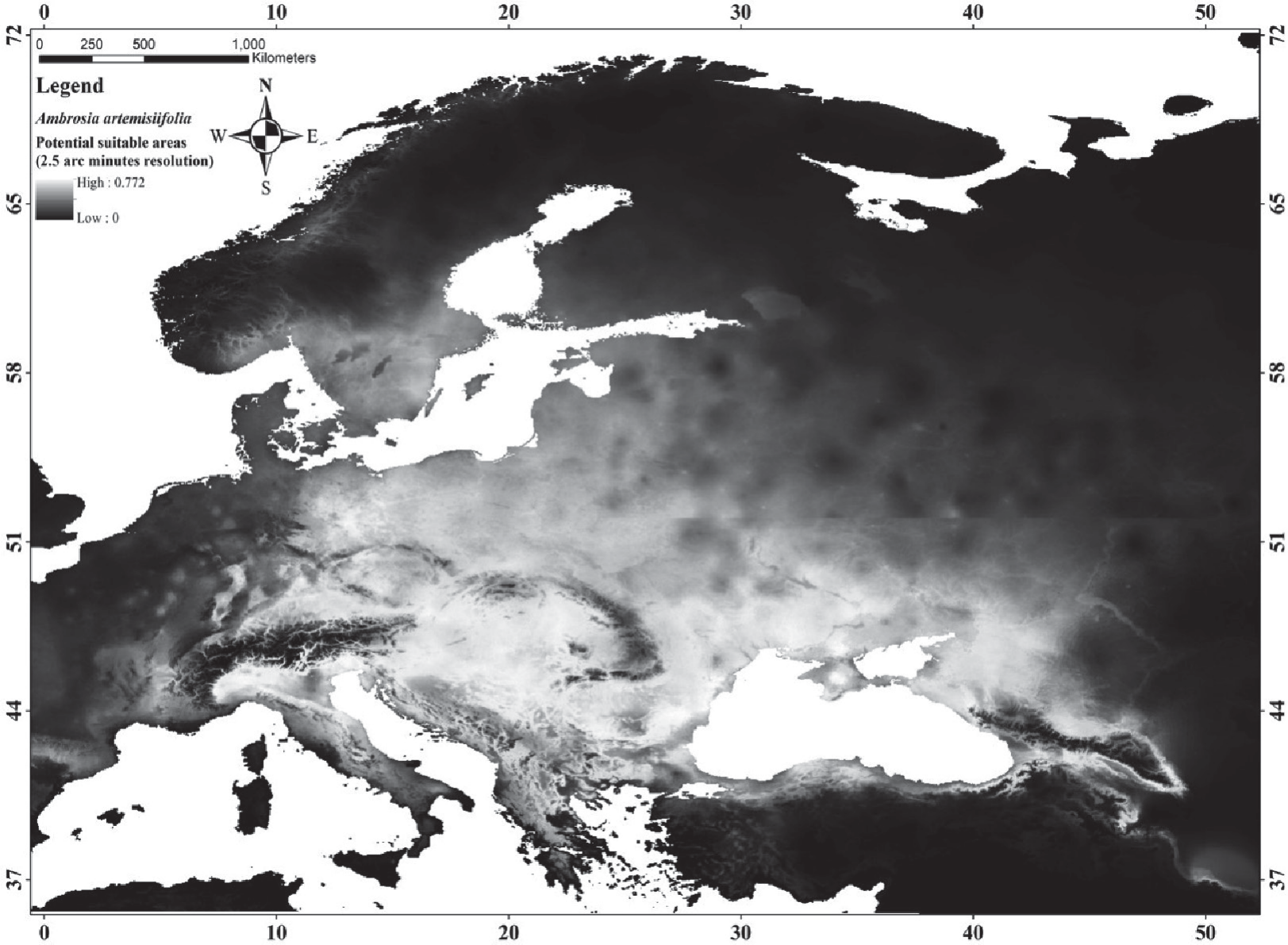
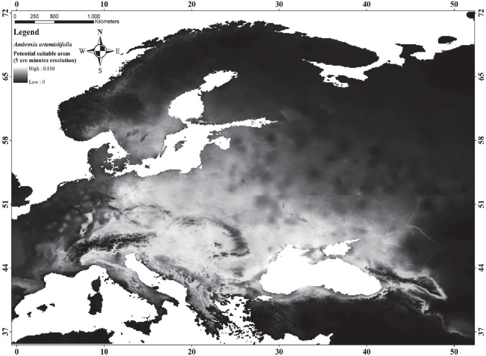
The Area Under the Curve (AUC) values also used for evaluation of the model performance [40]. As shown in Fig. 2, the AUC values are similar to the results obtained from the Kruskal Wallis test. The mean AUC values for the models with 25 arc minute, 5 arc minute, and 10 arc minute resolutions were determined to be 0.920, 0.934, and 0.950, respectively. All of the models, according to the classification system proposed by Swets (1988) [40], can be considered to be excellent (AUC≥0.90: excellent; 0.90>AUC≥0.80: good; 0.80>AUC≥0.70: fair). Based on these results, the most accurate model is the one that was created using bioclimatic variables at a resolution of 10 arc minutes (Fig. 2).
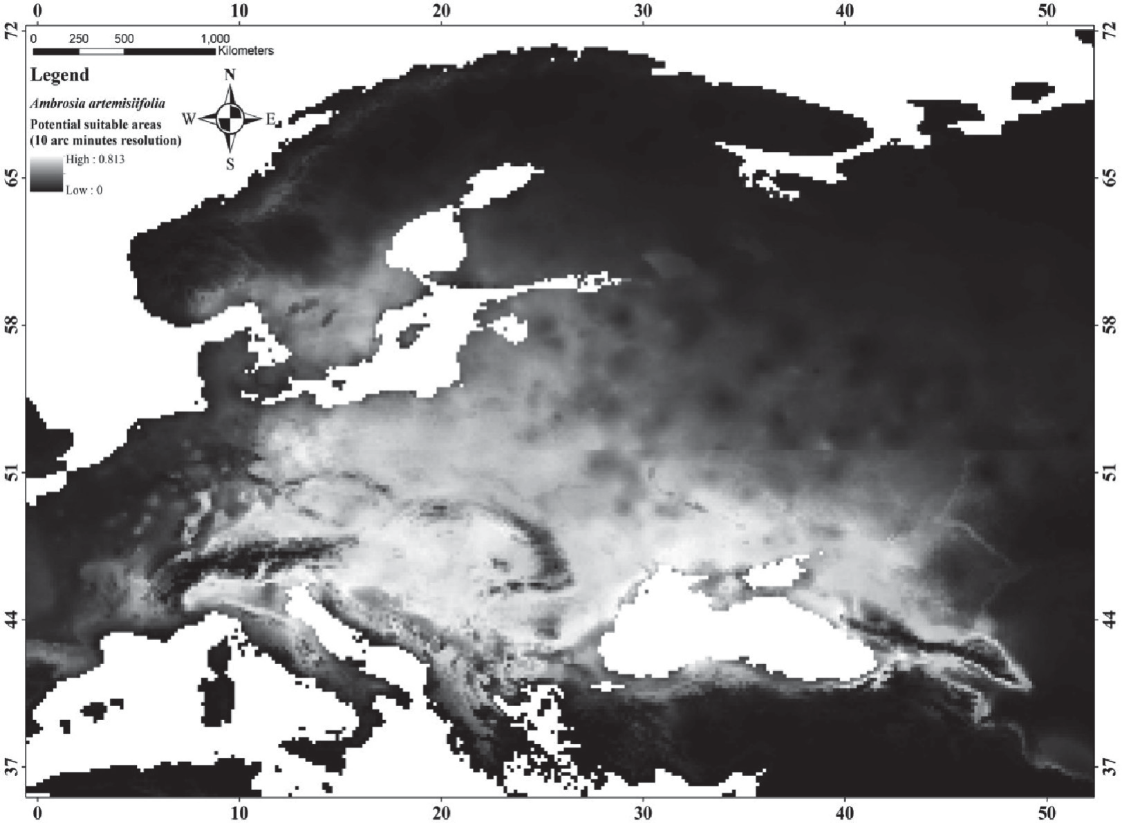
Within the scope of this research, the distribution of the species was modeled at different resolutions. The model with the highest AUC value of A. artemisiifolia has a resolution of 10 arc minutes. As can be seen in the distribution map of this model, the species has a wide distribution, similar to the studies given above. Especially north of Italy, central Europe, north and northwest of the Black Sea attract attention in terms of the distribution of the species.
Below are the potential distribution maps of the A. artemisiifolia obtained at three different resolutions, respectively (Figs 3-5). Potential distribution maps reveal that most of Europe represents potential suitable areas. Especially the northern part of Italy, Central Europe, Ukraine, Georgia, Western Russia, and the Black Sea region in the north of Türkiye are potential suitable areas. When the predictive values are thresholded according to the value of 0.5, suitable areas for 2.5, 5 and 10 arc minutes resolutions were determined as 1942000 km2, 1887000 km2, and 1781000 km2, respectively.
Results for Ailanthus altissima (A. altissima)
The second species modeled in the study is A. altissima. It is a deciduous tree indigenous to China. It was first brought to Europe and then to America towards the end of the 18th century. It is a widely cultivated and naturalized species in Europe, North America and Cyprus [41-42]. Currently, A. altissima has spread to all continents except Antarctica, and its distribution consists of areas between the temperate and meridional zones. As vertical distribution, it has a distribution from sea level to 2100 meters in North America, while in Europe it mostly occupies areas with a milder climate below 1000 meters. These features indicate that the ecological tolerance range of the species is quite wide [43-47].
Fig. 2.
AUC values of the model obtained for A. Artemisiifolia: a) 2.5 arc minutes, b) 5 arc minutes, c) 10 arc minutes.
A. altissima is used in the afforestation of unproductive areas in some regions, to combat erosion, and as a windbreak. Being a fast-growing species and having a high tolerance to environmental stress factors are the main reasons for its preference. On the other hand, it is also preferred in the paper industry because of its easy cellulose production [48]. Therefore, the aforementioned species stands out due to its chemical properties as well as its physical properties. All these features add positive points to the species. Moreover, some studies reveal that the species expands rapidly and grows more with increasing temperatures. Moreover, it often occupies low-maintenance areas. Hence, it is essential to be cautious so that this widely used species does not pose a threat to biodiversity. A. altissima is indicated to suppress native populations under suitable conditions, such as in Mediterranean regions. However, there is a lack of studies on its effects on natural environments. Mediterranean areas, characterized by typical Mediterranean vegetation like garigue and maquis, as well as shrublands, disturbed forests, grasslands, and riparian, mesic and xeric woodlands in southern and sub-southern zones, appear to be at the highest risk of A. altissima invasion [46]. Even, in some studies, it has been stated that A. altissima effects biodiversity negatively by reducing species richness (23.8 %±3.1 %) in the infested lands of Mediterranean islands, where it forms almost pure stands, and the highest effect is on therophyte species [49].
Fig. 6.
Group averages of the predictive values obtained from the models made for different resolutions of the A. Altissima.
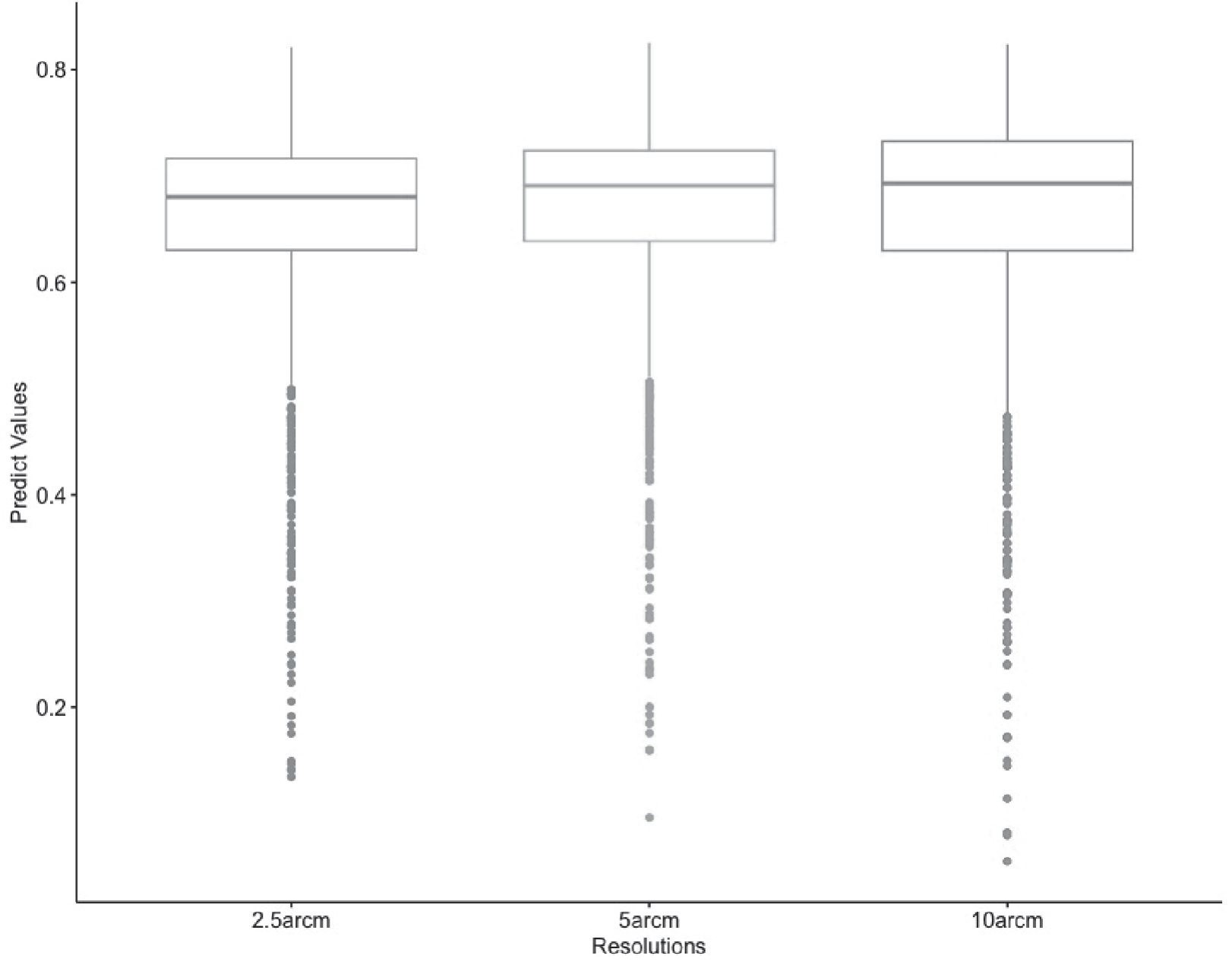
Fig. 7.
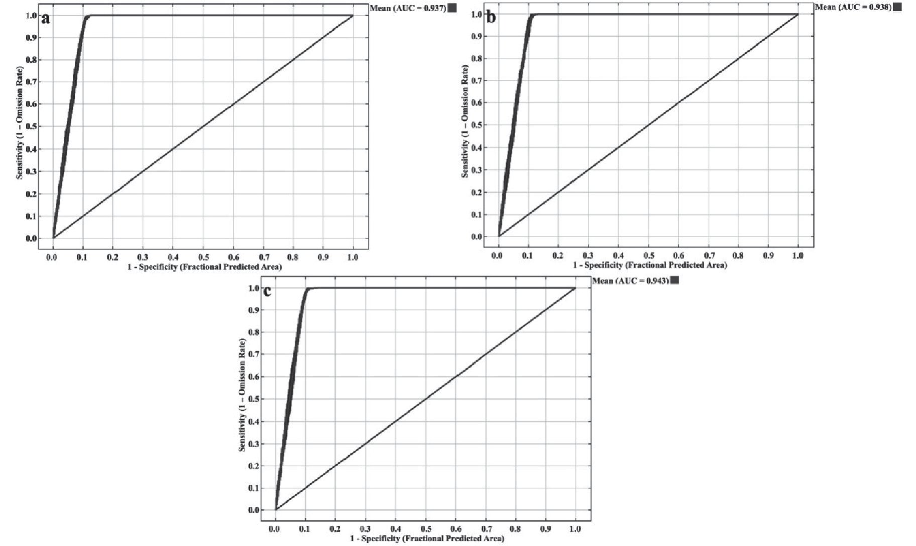
AUC values of the model obtained for A. Altissima: a) 2.5 arc minutes, b) 5 arc minutes, c) 10 arc minutes.
In addition to its impact on the environment, A. altissima also poses a significant threat to human health. Studies have shown that it can cause a range of health issues including dermatitis, allergic reactions, and in rare cases, myocarditis [47]. A study conducted in Sardinia found that 10 out of 54 patients with allergy symptoms were caused by A. altissima pollen. Other studies have also found that it can cause allergic reactions due to its high pollen production [50]. Additionally, contact with the sap of the plant can also cause dermatitis [51-52], and there have been a few cases of myocarditis reported in instances where sap entered the body through cuts or abrasions [53-54].
The results of the Kolmogorov-Smirnov normality test applied between the prediction values of the models made for A. altissima using bioclimatic variables with three different resolutions revealed that there was a significant difference in terms of the prediction values (p<0.05). That’s why, the Kruskal Wallis rank sum test was used, similar to A. artemisiifolia, in order to determine whether there was a difference between the prediction values. There is a significant relationship in terms of the Kruskal Wallis rank sum test results (p<0.05). However, the prediction values are quite similar in terms of group means (Fig. 6).
Distribution modeling of A. altissima was also performed for three different resolutions as in A. artemisiifolia. Similar results were obtained for A. altissima as well and the highest AUC value for A. altissima was determined to belong to 10 arc minutes resolution. It has been determined that as the resolution decreases, in other words, as the pixel size increases, the AUC value also increases. AUC values were determined as 0.937, 0.938, and 0.943 for 2.5, 5, and 10 arc minute resolutions, respectively (Fig. 7). According to Swets (1988)’s classification [24], all models obtained for A. altissima are excellent, as in A. artemisiifolia.
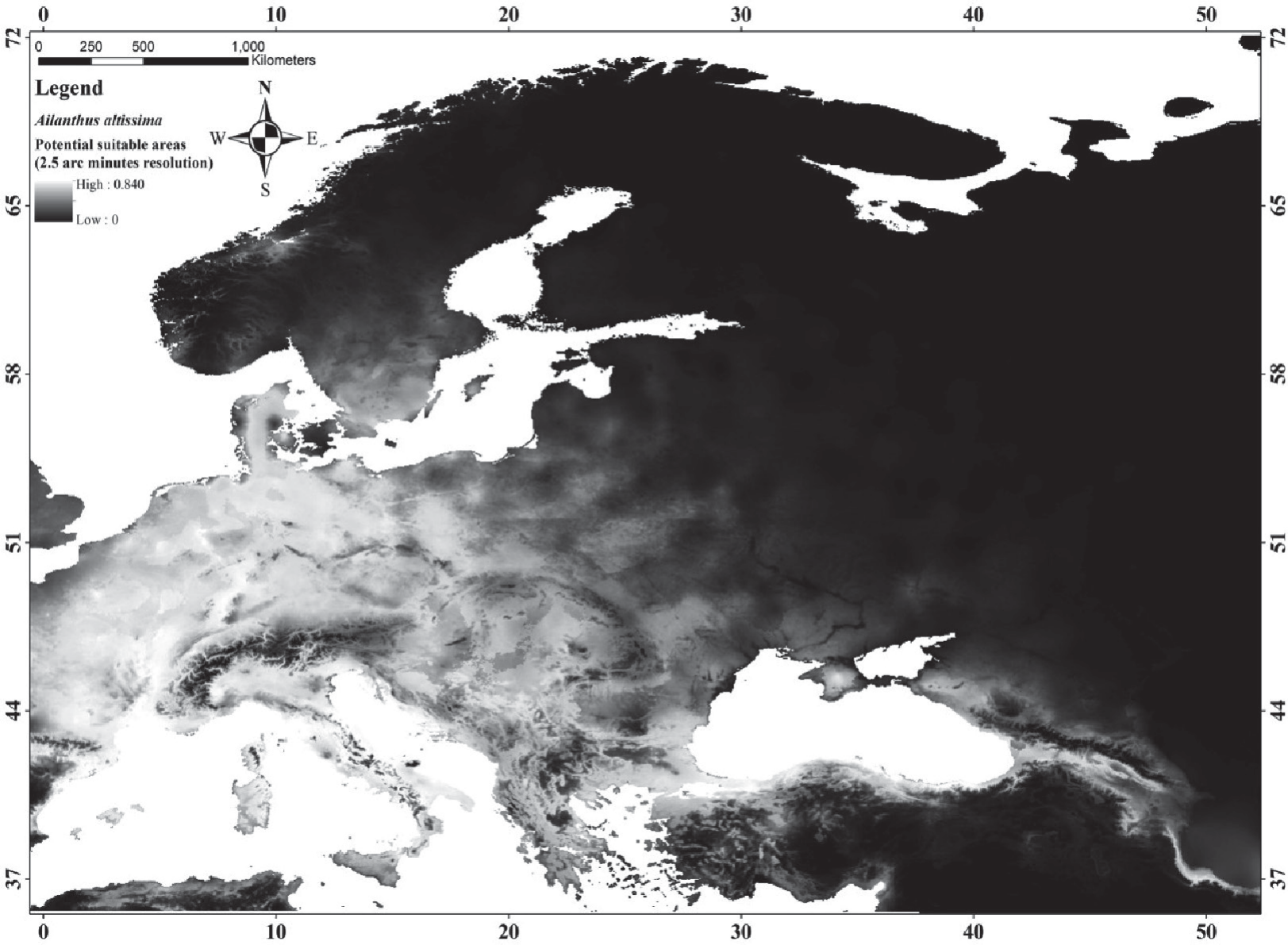
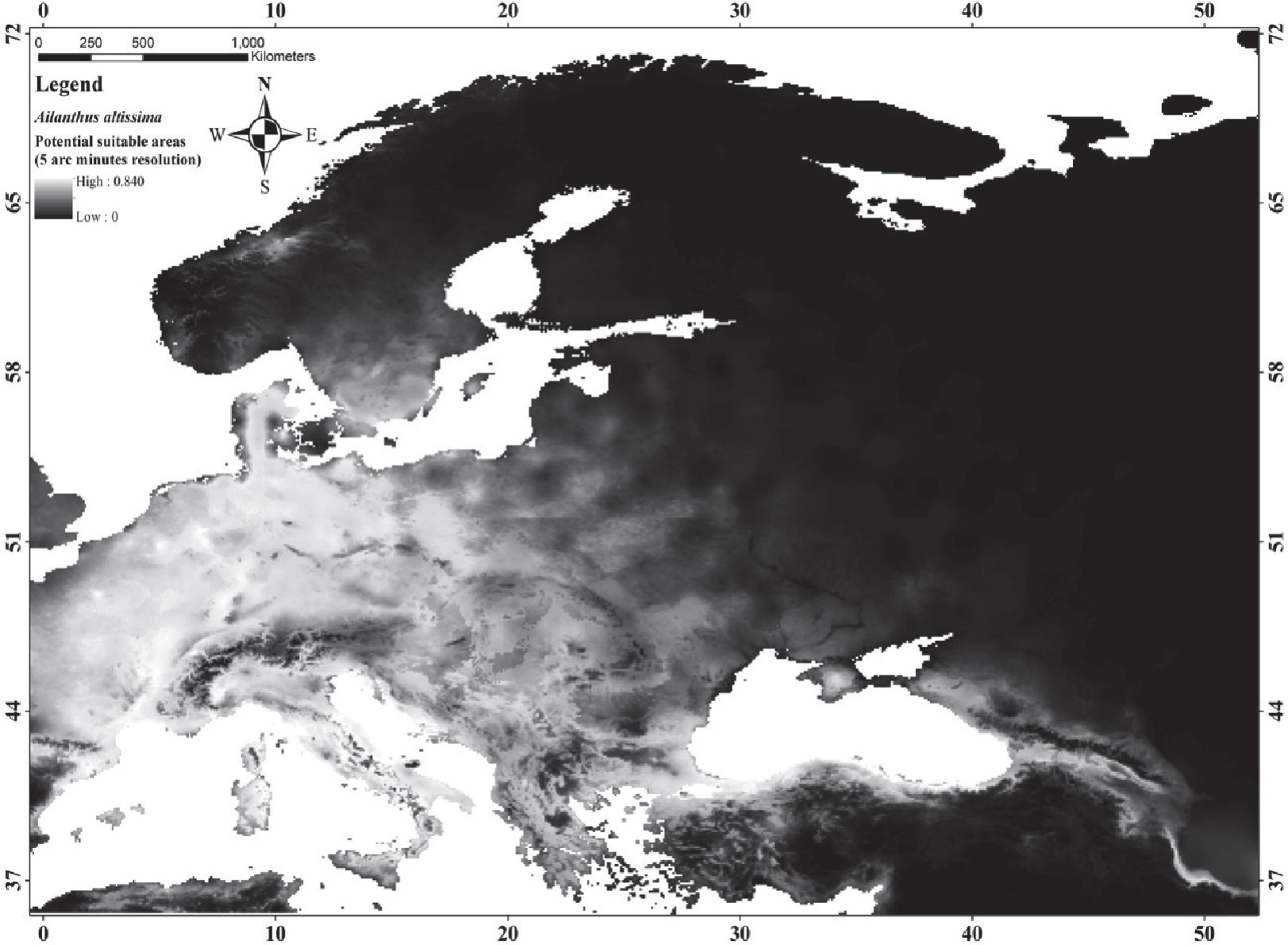
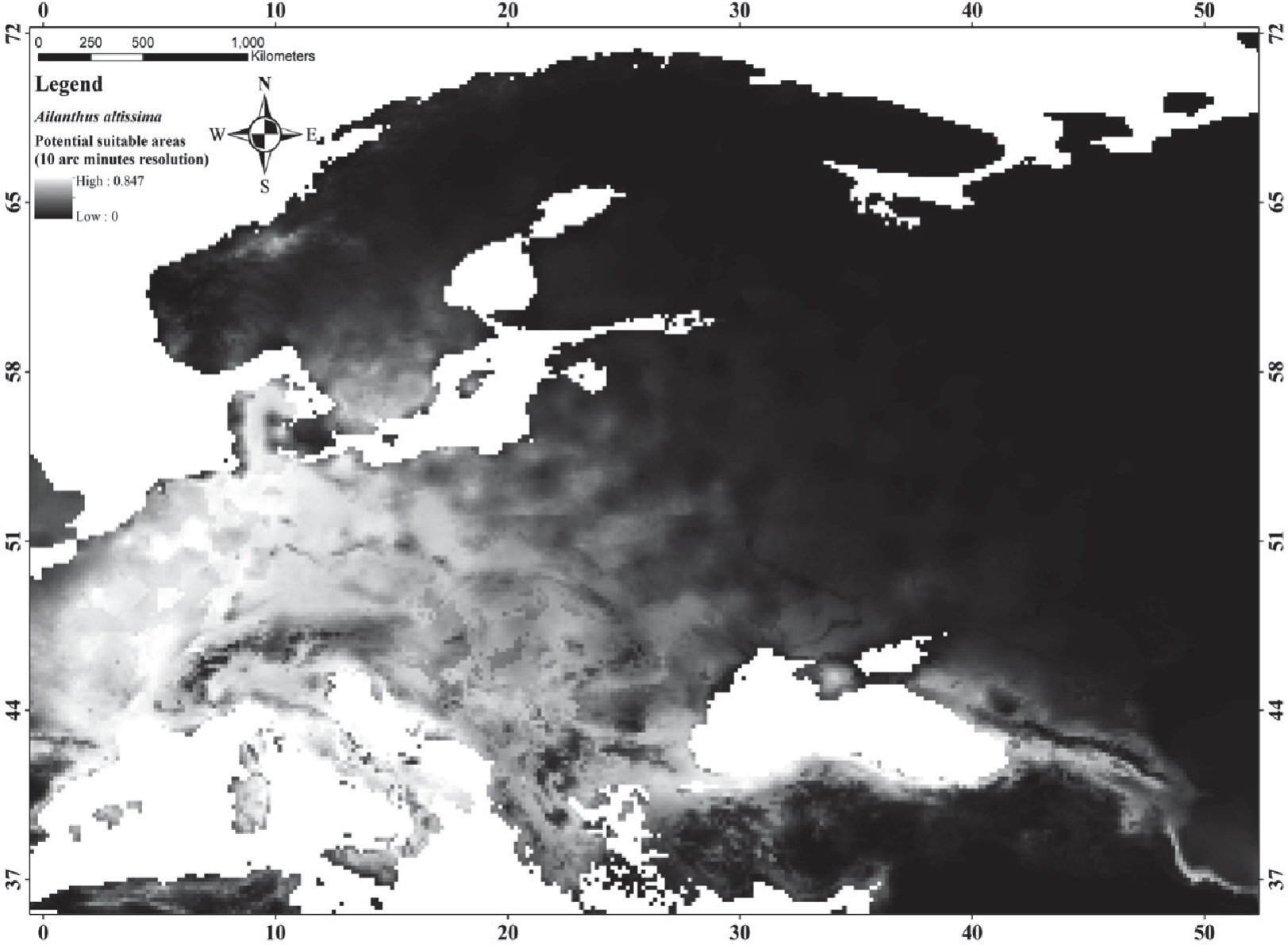
The predictive maps revealed a wide distribution of A. altissima. Potential distribution maps for Ailanthus altissima reveal that almost all of Europe and northern parts of Turkey represent potential distribution areas of the species (Fig. 8-10). Considering that 0.5 and above of the estimation values represent potential suitable areas, potential suitable areas were determined as 1628000 km2, 1662000 km2, and 1706000 km2, respectively.
Conclusions
The results of the study provided significant information on the effect of resolution on species distribution models. In line with this information, it was concluded that it would be more beneficial to work in large areas and to prefer bioclimatic variables with a resolution of 10 arc minutes in species with a wide distribution such as invasive species. In addition, it has been observed that the appropriate distribution areas of A. ailanthus and A. artemisiifolia, which are modeled as target species in the study, are quite wide. Considering the negative features as well as the positive features that cause these species to be preferred by humans will provide important positive outcomes in terms of parameters such as human health and biodiversity.