

Introduction
Despite being a significant form of pollution, noise pollution continues to be overlooked in numerous modern cities across the globe [1]. However, according to Fallah-Shorshani et al. [2] in recent years the issue of noise caused by traffic is becoming increasingly concerning. Because of that it requires a comprehensive and coordinated effort from all stakeholders to effectively address it and achieve the desired outcome of acceptable noise levels in different areas of the city [3]. Also, it should be noted that ambient noise and air pollution frequently appear together since they stem from identical origins, namely traffic [4], which is even more concerning because previous studies confirmed spatial connection between noise caused by traffic and air pollution [5]. In recent years, there has been an intensive development of air traffic, which in the areas located on the routes of airlines, and especially at airport locations, has led to environmental burdens to the upper tolerable limits. Although the aviation sector brings significant economic and social benefits [6] to the state, it also affects the increase in noise pollution and local air quality, as well as climate change [7]. The further growth of the aviation sector is directly conditioned by its efficient response to today’s major environmental challenges. The answers to these challenges must be environmentally sustainable and innovative, which is the only way to increase the competitiveness of the aviation sector in the global market [7]. The aviation sector is not fully comparable with other economic sectors, because the reduction of factors that affect environmental pollution in aviation is more difficult to achieve [8]. A full scientific understanding of the impact of aviation on the environment is an essential basis for discussing informed policy and for developing effective mitigation measures, which achieve the desired result in a cost-effective way.
Noise near airports is generated by aircraft movements, engine testing and other noise sources at airports, “en-route” aircraft flying and breaking the sound wall of supersonic aircraft [8]. The anxiety, which residents feel about a certain level of noise generated by air traffic, is greater than the anxiety caused by other means of transport [7]. Because of all the above, the fundamental goal of incorporating noise modeling in the process of evaluating environmental impact is to estimate the amount of noise that will be produced by a specific activity in the surrounding area [9]. This problem is especially pronounced when airports are located in the immediate vicinity of residential areas, hospitals and schools, as in the case of Mitiga Airport, which was the reason for conducting the research presented in this paper.
Geographic information system (GIS) has gained significant popularity and emerged as a pivotal evaluation tool in the field of ecological environment evaluation [10]. Because of that GIS was used during the research for generating noise maps [11] and graphical interpretation of the most polluted areas, based on measured noise levels (Lden) before and after the introduction of corrective measures and the creation of distribution maps. Graphical representation of these results in GIS is enabled by applying the Inverse Distance Weighting (IDW) interpolation technique. The IDW method is based on the assumption that the variable being mapped becomes less influential as the distance from its sampled location increases. It is particularly effective for the interpolating phenomena that exhibit a strong correlation with distance, such as air quality, water flow, and noise levels [12]. The decision to use IDW over alternative methods like Kriging was made on the assumption that IDW would result in a closer resemblance between the values of sample points and the values projected onto the cells [13]. This assumption is based on the idea that as a sample point gets closer to the cell being projected, the value of that cell would increasingly reflect the value of the sample point [13]. In contrast, Kriging estimates the intensity of unknown variables, without necessarily reducing intensity with distance [13]. Also, according to Ghojogh Nejad et al. [14], the IDW interpolation method better presents the mean values of the measured noise levels, compared to the Kriging method used to generate a map based on the maximum values of the measured noise levels. For this reason, the IDW interpolation technique was used in this study.
According to Olayode et al. [15], artificial neural networks (ANNs) can be characterized as a mathematical framework capable of conducting simulation analyses on the functional and structural components of biological neural networks. Neural networks can be described as mathematical systems that are capable of learning in a nonlinear manner [16]. Mansourkhaki et al. [17] believe that ANNs can be used more successfully comparing to traditional methods of data analysis and modeling [18]. Thanks to the latest progress in machine learning and the widespread access to enormous data collections, it is now feasible to create neural network models that can anticipate aviation noise based on the flight paths of airplanes [19]. In urban areas, traffic is the most prominent contributor to noise pollution which has a detrimental impact on human well-being, both physically and mentally, as well as work productivity [20]. Now, it is possible to create a predictive method by utilizing a range of detection devices to gather traffic data and incorporating historical traffic patterns and other significant variables [21]. Since ANN was already used in predicting air pollution [22], and it is also crucial to develop models that accurately predict the noise generated by air or road traffic [20], this was the reason why, in the final part of this paper, ANNs were used to assess the reliability of predicting noise levels generated by air traffic.
Due to all the above, the purpose of this research is to assess and reduce noise levels after the introduction of certain corrective measures to reduce the impact of noise at the specific airport Mitiga (Tripoli) in Libya, in order to present the distribution of noise levels in research and mark the most critical grids using various GIS techniques. Finally, the technique of ANNs, multilayer perceptron (MLP) was applied in order to assess the reliability of predicting the level of noise generated by air traffic, and the results were compared with the results of multiple linear regression (MLR) models to confirm the reliability of noise level prediction using ANN method.
Materials and Methods
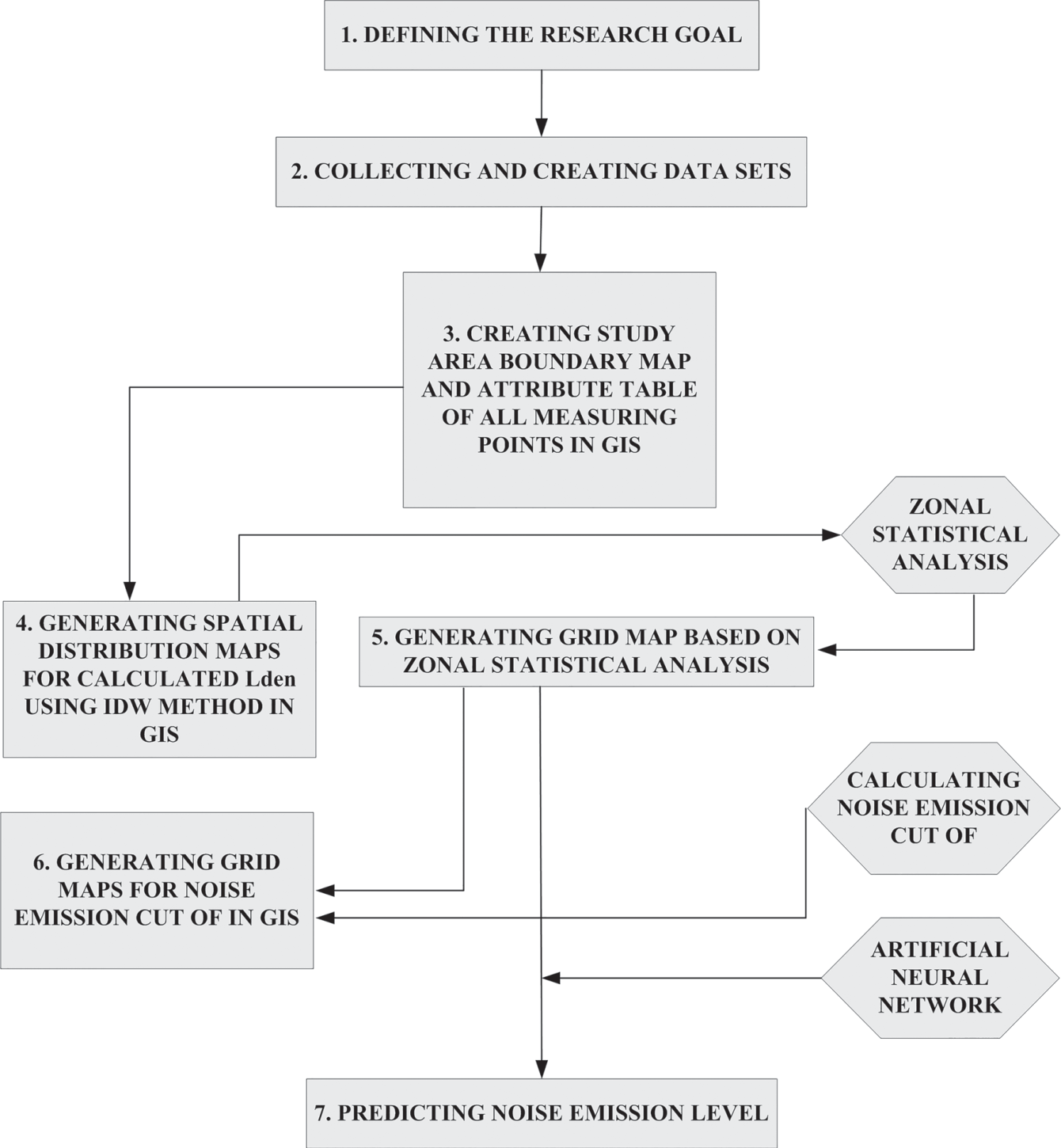
A model for estimating, reducing and predicting noise emissions has been created in order to enable the most efficient management of this environmental pollutant. The model consists of seven steps (Fig. 1).
The first step was defining the research goal – estimating, reducing and predicting noise emissions caused by aircrafts. The second step was collecting and creating data sets – in this step noise emissions were measured at three locations within the research area, before and after the introduction of measures to reduce noise emission generated by air traffic. The third step was creating study area boundary map and attribute table of all measured points in GIS – in this step a database was created in GIS, which contains all the necessary data on measuring points and measured noise emission (Lday, Levening, Lnight and Lden) before and after the application of reduction measures. The fourth step was generating spatial distribution maps for calculated Lden using IDW method in GIS – in this step the IDW method in GIS was used for creating interpolation maps of the research area with measuring points, in order to graphically present the distribution of noise emissions before and after the introduction of certain corrective measures. The fifth step was generating grid map based on zonal statistical analysis – in this step the investigated area was divided into 16 grids (4x4) and zonal statistics applied to the data before and after the introduction of certain measures. The sixth step was generating grid maps for noise emission cut of in GIS – the results of zonal statistics were used to calculate the noise level in each control grid before and after the application of reduction measures, based on which the mapping of grid according to the level of noise pollution was performed. Finally, the seventh step was predicting noise emission level – in this step ANNs have been used to assess the reliability of predicting noise levels in the research area.
Research Area
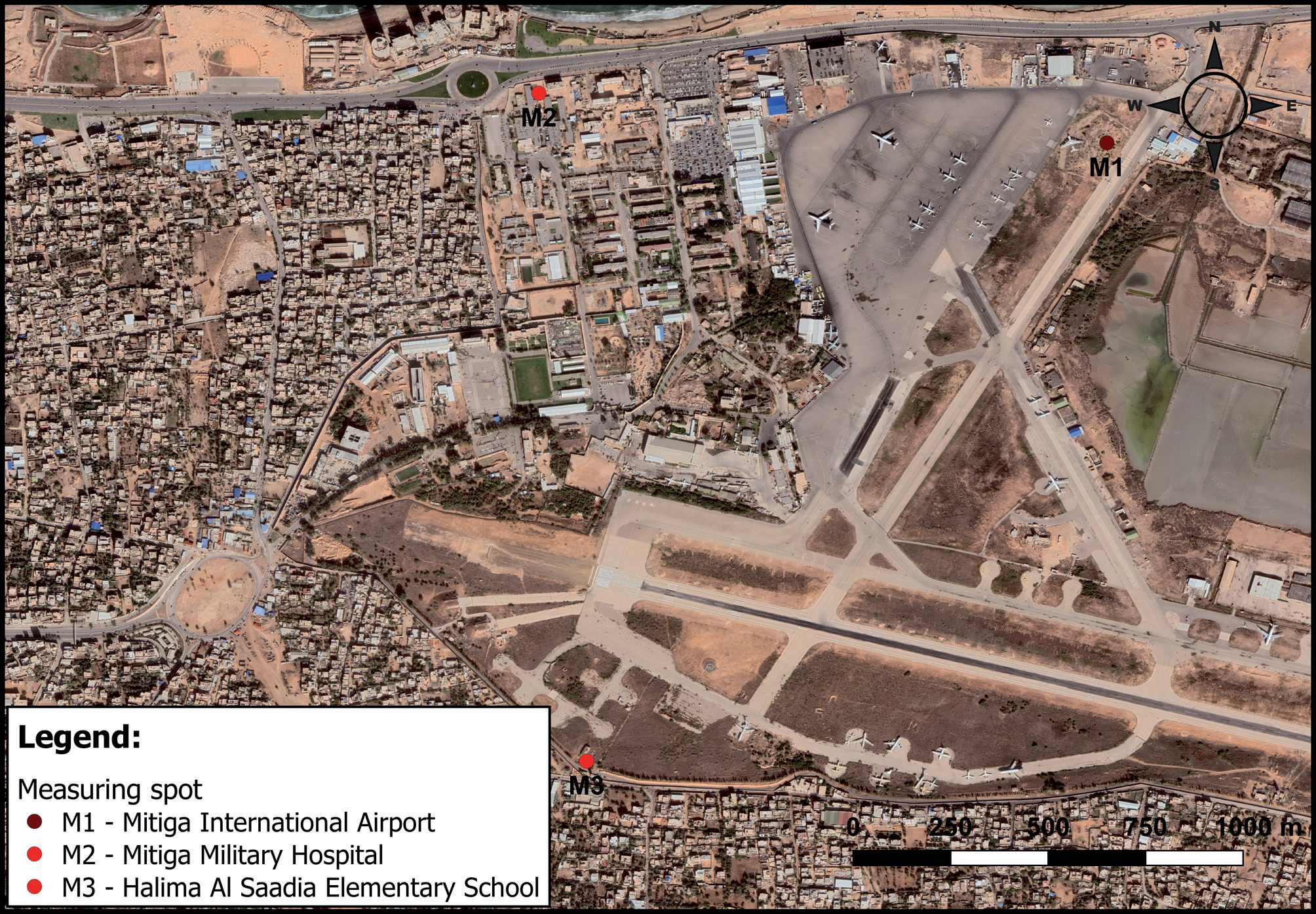
The area of research is Mitiga International Airport in Libya (13o16’40”E, N32o53’40”N, elevation 11 m) (Fig. 2). This airport is located in the municipality of Tripoli, the capital of Libya. The planes operating on these routes are Airbus 320, Airbus 319, Airbus 321, Airbus 332, Boing 738, Boing 734, CRJ9 and ERJ145. The runway has an asphalt surface and has a length of 3,400 m. Near the airport are Mitiga Military Hospital (13o16’08”E, 32o54’25”N, elevation 10 m) and Halim Al Saadia Elementary School (13o16’12”E, 32o53’29”N, elevation 11 m).
In the period when the noise level was measured, there were an average about 43 landings and take-offs per day. Noise level measurement was carried out in the period of June, July, August 2021, and cases of approximately the same engine power were analyzed. Phase 1 was from June 1 to July 15, 2021, and Phase 2 from July 16 to August 31, 2021. The total number of flights in the observed period is: June 1,363; July 1,364 and August 1,242.
Therefore, measurements were made continuously for 3 months, 24 hours a day (except for the school location). The measurement was carried out in the period from June 1 to August 31, 2021, because it was observed that in that period, although the traffic frequency was not the highest in 2021, it was the highest in previous years. It was not possible to perform longer-term measurements, because this research was conducted only as a part of the student’s doctoral dissertation. As a result, the obtained Lden values are more conservative and higher than the actual ones. The noise level was measured with three sensors of the same type, which were placed at locations M1, M2 and M3 (Fig. 2).
Given that airborne noise has an impact on the health of people living near the airport, as it affects sleep disorders, cardiovascular diseases, including hypertension, altered cognitive abilities in children, preterm birth, hormonal disorders [23, 24, 25], and higher risk of metabolic syndrome [26], the research idea was to determine the noise level in the area that would include these three locations and to implement measures to reduce noise levels in accordance with the measurement results, the effect of which would be determined by a new set of noise measurements, at the same locations.
Measuring of the Noise Level
During three-month period (from June until September in 2021.) noise levels were measured at three locations near the runway threshold 10 (13°16.22’E, 32°53.75’N) (Fig. 2): – M1 (measuring spot 1) - at Mitiga Airport, where the
airport staff is about 1,500 m away from the runway
threshold 10 (13o16’40”E, N32o53’40”N), – M2 (measuring spot 2) - in the military hospital
Mitiga, which is at a distance of 1,225 m from the
runway threshold 10 (13o16’08”E, 32o54’25”N) and – M3 (measuring spot 3) - Halima Al Saadia Primary
School, which is 550 m from the runway threshold
10 (13o16’12”E, 32o53’29”N).
Measurement of noise levels at all three locations was done for the peak load of the airport (the largest number of take-offs and landings of aircraft that generate high noise levels). Also, the measurements were performed in two phases: (1) before the introduction of noise reduction measures and (2) after the introduction of noise reduction measures.
These measures were implemented as a test for this research, which lasted from July 16 to August 31, 2021. The airport authorities have built barriers made of brick and aluminum. All airlines that used the airport in the specified period, as well as ATC (air traffic control), participated in the introduction of the measures.
The impulse precision sound level meter B&K 2209, manufactured by Brüel & Kjær, was used to measure the noise level, and the measurement was performed during three periods, during the day (from 7 h to 19 h), in the evening (from 19 h to 23 h) and at night (from 23 h to 7 h) at the airport and hospital, while at the school location, the measurement was performed only during two periods, during the day and in the evening (the measurement was not done at night, because at the time the school was closed).
One of the goals of this paper is to determine the spatial distribution of 24-hour noise emissions (Lden) generated by air traffic at Mitiga Airport (Tripoli, Libya) using GIS methodology, in order to identify noise pollution levels in relation to the location of Mitiga Military Hospital and Halim Al Saadia Elementary School located near this airport. Due to the fact that noise was measured at three measuring points, during the day, evening and night, 24-hour noise emissions (Lden) had to be calculated using “the following formula [27, 28]:
where: – Ld is the A-weighted long-term average sound level
determined over all the day periods of the year, – Le is the A-weighted long-term average sound level
determined over all the evening periods of a year,
and – Ln is the A-weighted long-term average sound level
determined over all the night periods of a year” [27,
page 252].
Mihajlov and Prascevic [27] used noise indicators Ld, Le and Ln to present daily, evening and night noise indicators (Lday, Levening and Lnight).
The Guideline Development Group (GDG) of the World Health Organization (WHO) has suggested that the noise levels produced by aircraft should be reduced to levels below 45 dB Lden and 40 dB Lnight during night time as it can have negative effect on health and sleep [29]. The GDG has also expressed its confidence in the fact that exposure to noise levels below 45 dB Lden can lead to an increased risk of annoyance [29]. We noticed that these threshold values are about 10 dB lower than the threshold values in the EU member states, so we increased the WHO limit values for Lden and Lnight by 10 dB and conducted this research with a limit value of Lden = 55 dB and Lnight = 50 dB.
Noise at the school location was measured only during the day and evening, because the school does not work at night, so when calculating the Lden value for a given location for Lnight, a limit value of 50 dB was taken into account. The pupils are not affected by noise during the night, since the school is closed, but the people living near the school are. Since the aim of our research was to assess the noise impact on pupils who are attending school near Mitiga airport, not the people living nearby, we did not measure noise during the night at the measuring spot M3, but we assumed that it was within the limit value (50 dB), and the sensitivity analysis have shown that the results for Lden would not differ much in case that the values for Lnight are equal to 0 dB. Besides, in reality outdoor noise value at night is never 0 dB. This is why we used the limit value for Lnight = 50 dB. Although, if the noise was measured during the night period in the measuring spot M3, the values would certainly be higher than 50 dB, as well as the calculated Lden values.
It was assumed that the noise at the M3 measuring point at night would be greater than 50 dB because it is close to the runway, and the noise level measured at the M2 measuring point is the farthest from the runway before and after the introduction of noise reduction measures, was greater than 50 dB. Also, it is a well-known fact that the noise is decreasing by increasing the distance. The sensitivity analysis was done separately for the measurement results before and after the introduction of noise decrease measures. The value for the M3 measuring point at night was increased by 10 and 20% to get the value for Lnight as closest to the mean noise value measured at the measuring point M2 at night which according to the results in Table 1 was 58.04 dB.The results have shown that in this case values for Lnight would be 55 dB (increased by 10%), and 60 dB (increased by 20%), and the calculated mean values for Lden would be 70.78 dB and 71.80 dB, respectively. The same analysis was done for the measurements after the application of noise decrease measures. However, since the mean noise level at measuring point M2 at night (Table 2) in this case was 51.34 dB, it was necessary to increase noise at the M3 measuring point at night by 2.5 and 5%, thus the new values for Lnight would be 51.25 dB (increased for 2.5%) and 52.5 dB (increased for 5%). New calculated mean Lden values for the M3 measuring point were 58.64 dB and 59.45 dB, respectively. As can be seen, the sensitivity analysis has shown that by increasing the Lnight values, the Lden values will also be higher. However, the influence of increased Lnight values on mean Lden values at the M3 measuring point will not be so big, as can be seen by comparing with the results for calculated mean Lden values at the M3 measuring point (Tables 1, 2).
Geographic Information System
Fig. 2 shows a map with three locations where noise was measured (measuring points M1, M2 and M3). This map was created in GIS, using the QGIS software package (version 3.6). Since GIS has a very powerful spatial analysis capabilities [30, 31], it was used to create layers that contain all the necessary information for segmenting grids based on the boundaries of the research area. The research area consisted of 4x4 grids covering an area of 5.968 square kilometers. It has also been considered dividing the area into different numbers of grids but the results were not significantly different. In order to generate noise levels per grid, the measured noise values (Lday, Levening and Lnight) were used to calculate the 24-hour noise (Lden) measured at three locations and these results were then used in zonal statistics in GIS. The spatial distribution of noise emission was calculated using the IDW interpolation method, and the previously calculated Lden values for all three measuring points. IDW interpolation method [32] was used in this study to show the spatial distribution [33] of noise emission. The IDW method generates maps that offer valuable information for monitoring purposes, even when only a small number of monitoring units are available [34]. This is one of the simplest methods based on the assumption that the value at an uncompressed point can be approximated as a weighted average of values within points within certain distances or from a given number of the nearest points (usually 10 to 30) [35]. The weights are usually inversely proportional to the distance [27], which leads to estimation in an unspecified location. Therefore, the interpolation is calculated as follows [36]:
Table 1.
Descriptive statistics of the measured noise emission caused by aircrafts before the introduction of measures.
Table 2.
Descriptive statistics of the measured noise emission caused by aircrafts after the introduction of measures.
where m represents the number of the nearest points, r location, and p represents the parameter [36].
After applying the IDW interpolation method and creating spatial distribution maps [37] of noise emission and obtained average Lden values per grid, using zonal statistics as table tool in GIS, deviations from the limit value in each grid were calculated, assuming that the limit value for Lden is 55 dB.
Artificial Neural Networks
ANN technology was used to assess the reliability of noise level prediction [17]. This technique was used within the SPSS software package (version 20) and on that occasion the MLP structure of the neural network was used as one of the most commonly used ANNs. MLPs include input layer, hidden layer and output layer [38], and in this study they were used to predict variations in noise levels. Each MLP had one output (Lday, Levening, Lnight, or Lden) and three inputs (engine power, take-off and landing runway distance, and air traffic volume) that were used to identify differences between noise measurement locations. The training, validation and testing phases play a crucial role in the field of machine learning [39]. During the training phase, the corpus was organized in a manner that aligns with the algorithms’ computational requirements. This allows the model to learn from their trial and error experiences. To ensure comprehensive training, the dataset was divided into three segments, so when defining MLPs, it was determined that 70% of the sample would be random selection for training, i.e., calibration model, 20% for testing and 10% for model validation. Ratio 70:20:10 was also used by other authors like Zhang et al. [40], Kowsher et al. [39] and Karpathy et al. [41]. As Kowsher et al. [39] stated the training segment, comprising 70% of the dataset, was utilized to train the models. The testing phase involved using the remaining 20% of the dataset as a dedicated testing set to assess the models’ performance [39]. Lastly, 10% was set aside for validation, aiding the models in evaluating their own performance and facilitating iterative improvements during the training process [39]. A training dataset for an ANN can have any number of hidden layers, which can also have any number of neurons [42]. Until the sum of the square error of the training template reached the minimum, the training is performed. The MLP analysis in this research was done based on 198 samples (for training, testing and holdout) for all outputs except for Lnight (132 samples) because the measurement was not done during the night period. To assess how well the ANN models are performing in terms of precision, the criterion used is the root mean square error (RMSE). The RMSE is calculated using the following equation [16]:
where Oi is the observed value and Pi is the computational value. The n parameter represent the number of data.
Multiple Linear Regression
MLR method was also used in predicting noise pollution levels at Mitiga International airport in Tripoli, in order to compare the results achieved by ANN method with another traditional model like MLR.
The equation for multiple linear regression for k variables used for calculating noise pollution levels in the research was [43]:
where the dependent variable i.e. noise pollution levels (Lday, Levening, Lnight and Lden) is y; coefficients of the regression evaluation are β1, β2 and βk while β0 is the y-intercept (value of y when all other parameters are set to 0); xi values are independent variables (runway distance (RD), air traffic volume (ATV) and engine power (EP)); ei is model error.
Results and Discussion
Descriptive statistics for all measured noise emission values (Lday, Levening, Lnight and Lden) at all three measurement locations are shown in Table 1 and Table 2.
In Table 1 Skewness values are negative for all noise indicators except for measuring spot M2 (for noise indicator Levening) where it is positive and greater than zero. Negative Skewness values mean that the noise emission has a longer left tail distribution, while positive and greater than zero Skewness values mean that the noise distribution of the test area is asymmetric. All Kurtosis values (Table 1) are negative, which means that the noise emissions also have a light-tailed distribution. Additionally, it should be noted that the noise was not measured at night at the measuring spot M3 (in both cases, before and after the introduction of measures), considering that the school is closed during night hours, so the descriptive statistical analysis was not made for noise indicator Lnight.
In Table 2 Skewness values are positive for measuring spot M1 (for all noise indicators), while negative for measuring spots M2 (for all noise indicators) and M3 (for all noise indicators except noise indicator Lnight). The Kurtosis values are all negative.
Considering that the maximum noise emission level for all four parameters was 81 dB and higher, it was determined that it is necessary to take certain measures to reduce the noise emission levels caused by air traffic. In this sense, after the first phase of measurements, the following measures were introduced to reduce noise emissions: – Engine power was reduced during take-off (from
92.8% and 83% to 83% and 80%, respectively); – Engine power at landing remained at 38%, but the
speed of the aircraft was reduced to the lowest
possible; – An aluminum partition has been installed at one
end of the runway threshold 10, towards the hospital.
The thickness of this barrier is 2 mm, the length
is 750 m, and the height 2 m. The aluminum barrier
is 232 m away from the hospital; – Another, brick partition was set up towards the
school, almost parallel to the runway. The thickness
of the masonry partition is 40 cm, the length
is 825 m, and the height 4 m. The masonry barrier
is 26 m away from the school; – The flight procedures in the take-off phase (on
departure) have been changed. On departure
there are two noise abatement procedures where
a stepped departure climb is being used. They are
called “NADP 1” and “NADP 2” (Noise Abatement
Departure Procedures). NADP 1 is used where there
are noise sensitive areas close to the airport and is
used to alleviate noise in an area further away, say
+25 km from the start of roll on the airport runway.
The restriction to two noise abatement departure
procedures was agreed at the ICAO (International
Civil Aviation Organization) in order to minimize
confusion internationally at the appropriate
procedure to use for the lessening of noise for people
on the ground. Essentially the two noise abatement
procedures are: – NADP 1: Aircraft to climb to 800’+ and then reduce
thrust. Keep flaps lowered in take-off mode and
continue climbing as fast as possible to 3,000’. Then
retract flaps, increase thrust and go on their way; – NADP 2: Aircraft to climb to 800’+ and then reduce
thrust. Withdraw flaps at that point and continue at
a decreased rate of climb until 3,000’ Then increase
climb and thrust and go on their way. – The NADP 1 procedure was applied in the research.
Application of GIS
After all measurements were performed both before and after the introduction of corrective measures to reduce noise levels, at all three locations, the data were entered into the GIS database for further analysis. First, based on the entered data on measured values and the application of the IDW interpolation method (Equation 2), maps of noise emission distribution were created before and after the introduction of corrective measures (Fig. 3).
It is noted that the noise level was significantly higher before the introduction of corrective measures (Fig. 3a), with the lowest noise emission values (from 59.02 dB to 70.30 dB) recorded in the military hospital (M2), while in the school area (M3) recorded values were between 63.28 dB and 75.29 dB. The highest values of noise emission were measured in the area of the airport (M1) and ranged from 76.07 dB to 87.90 dB. After the introduction of corrective measures (Fig. 3b), the noise emission values in the hospital area (M2) ranged from 55.72 dB to 59.65 dB, in the school area (M3) between 56.96 dB and 58.94 dB. The highest noise level was still in the area of the airport (M1) and ranged between 59.99 dB and 63.76 dB.
The distribution maps shown in Fig. 3 indicate that the area around Mitiga Airport and the population living in that location are still exposed to noise above 55 dB. According to Souza & Zannin [44] exposure to noise above 55 dB can reflect the health of the population living nearby [45]. Also, Baloye and Palamuleni [46] stated that noise sensitivity zones with noise level between 50 dB and 60 dB are considered risky, between 60 dB and 65 dB moderately risky, between 65 dB and 70 dB highly risky, between 70 dB and 75 dB dangerous, between 75 dB and 80 dB highly dangerous, while noise levels above 80 dB are extremely dangerous.
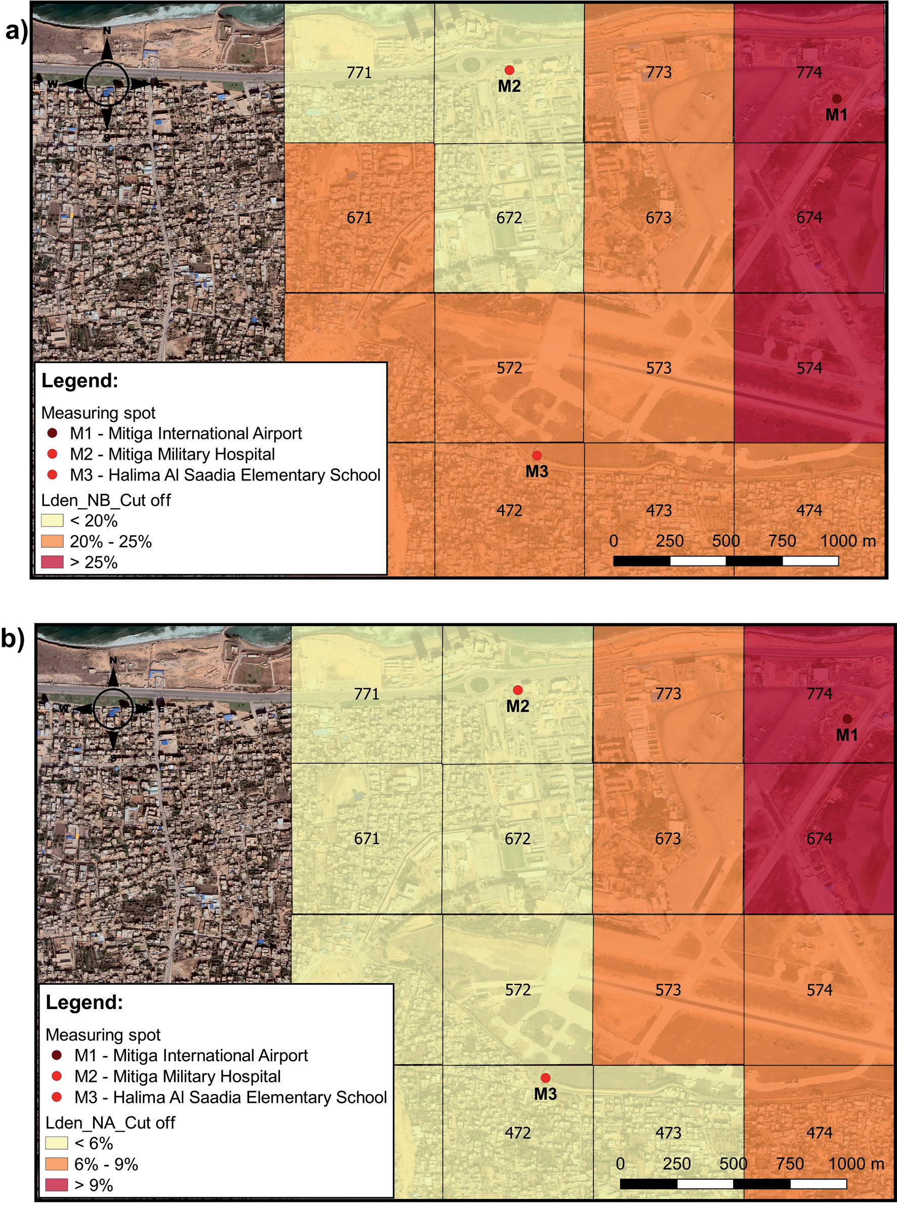
After creating maps of spatial distribution of noise emissions, the investigated area was divided into 16 grids and zonal statistics as table tool in GIS was applied for calculating deviations from the limit value for each grid. Then these deviations were entered into the GIS database and maps were created showing the deviations from the limit values per grid. Deviations from the limit values were calculated for Lden before and after the introduction of corrective measures (Fig. 4).
As can be seen in Fig. 4a), before the introduction of corrective measures less than 20% deviations was on the following grids: 672 (19.94%), 771 (18.43%) and 772 (16.91%), between 20% and 25% deviations was on the grids: 471 (22.05%), 472 (21.96%), 473 (22.55%), 474 (24.32%), 571 (21.65%), 572 (21.88%), 573 (23.22%), 671 (20.02%) ) and 673 (24.54%), while over 25% of the deviations were on the grids: 574 (26.28%), 674 (30.21%) and 774 (31.96%). Regarding deviations after the introduction of corrective measures (Fig. 4b), less than 6% of deviations were on the following grids: 471 (5.48%), 472 (5.19%), 473 (5.58%), 571 (5.58%), 572 (5.37%), 671 (5.68%), 672 (5.73%), 771 (5.53%) and 772 (5.22%), between 6% and 9% deviations were on the grids: 474 (6.65%), 573 (6.10%), 574 7.70%), 673 (7.33%) and 773 (7.45%), while more than 9% of the deviations were still on the grids: 674 (9.66%) and 774 (10.50%).
All deviations from the limit value of noise levels used in the research, before and after the introduction of measures to reduce noise levels caused by air traffic are shown in Table 3.
As can be seen from Table 3, after the application of certain measures to reduce noise levels caused by air traffic, a significant reduction in noise emissions was achieved, but it is also noticeable that it is necessary to introduce additional measures to keep noise levels within limits, i.e. below 55 dB.
For this reason, the following additional measures have been proposed, which can be applied in the research area: – planting trees in the immediate vicinity of the school
and military hospital, – implementation of the so-called green roofs on both
buildings, – thicker facade of buildings and replacement of
windows and doors (sound insulation), etc. –
Application of ANNs
In order to assess the reliability of predicting the emission of the examined parameters (Lday, Levening, Lnight and Lden), i.e., to achieve the second goal of the research, the method of ANNs, i.e., MLP was used. Input, i.e. independent variables of this model included: engine power (%), runway distance (m) and air traffic volume, while the dependent variables included noise emission parameters (Lday, Levening, Lnight and Lden).
The results of ANN analysis for all four outputs (Lday, Levening, Lnight, or Lden) are presented in Table 4.
The results in Table 4 show that in all cases, ie. for all four outputs (Lday, Levening, Lnight, or Lden) RMSE values are lower than 1 which implies a higher coefficient of determination (Figs 5-8). RMSE is a performance metric that provides information about the short-term efficiency of a model. It measures the difference between predicted values and observed values, with a lower RMSE indicating a more accurate evaluation. On the other hand, the coefficient of determination (R2) measures the variance explained by the model, reflecting the reduction in variance when using the model. R2 ranges from 0 to 1, with a value close to 1 indicating a model with strong predictive ability and a value close to 0 indicating a model that is not effective in analyzing the data. These performance metrics, RMSE and R2, are reliable measures of the overall predictive accuracy of a model [47]. Accuracy metrics are commonly used in ANNs to assess the quality of predictions. Beside Mean square error (MSE), mean absolute error (MAE), mean absolute percentage error (MAPE), and symmetric mean absolute percentage error (SMAPE), RMSE is widely used accuracy metrics in various fields such as weather forecasting, medical, and engineering [48]. RMSE, specifically, measures the average magnitude of error between predicted and actual values. It can be visualized as the average vertical distance from the actual value to the corresponding predicted value on a fitted line. In simple terms, RMSE is the square root of MSE. Similar to MSE, the range of RMSE is from 0 to positive infinity, and a smaller RMSE value indicates a higher accuracy of the prediction model. However, unlike MSE, the units of RMSE are the same as the original units, making it more easily interpretable [48].
Fig. 3.
Lden distribution maps: a) noise before corrective measures (Lden_NB) and b) noise after corrective measures (Lden_NA).
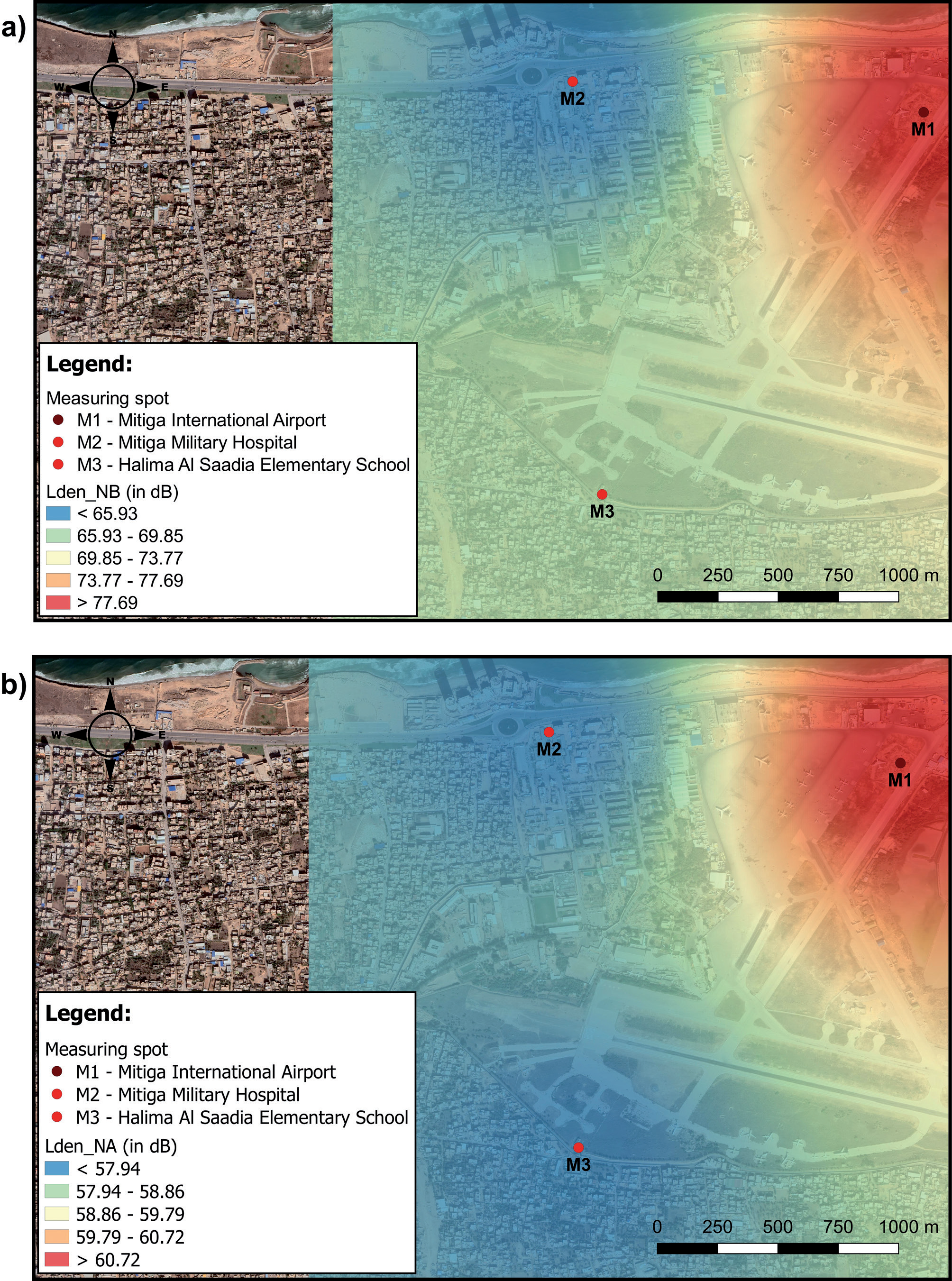
Fig. 4.
Lden cut of scheme: a) noise before corrective measures (Lden_NB_cut off) and b) noise after corrective measures (Lden_NA_cut off).
The assessment of the reliability of the prediction using MLP showed that changes in noise emission during the day (Lday) in the study area resulted in a coefficient of determination of 0.996 (Fig. 5a). As can be seen on Fig. 5a, the distinction between the actual values and the predicted values was in range of -2.04 to +1.32 dB. Significance analysis (Fig. 5b) showed that air traffic volume has the greatest impact on predicting Lday variations.
The assessment of the reliability of the prediction of noise levels in the evening (Levening) resulted in a coefficient of determination of 0.997 (Fig. 6a) and that the difference between the actual values and the predicted values was in range of -1.55 to +1.40 dB, while the significance analysis (Fig. 6b) showed that air traffic volume has the greatest impact on predicting Levening variations.
The assessment of the reliability of the prediction of noise levels at night (Lnight) resulted in a coefficient of determination of 0.997 (Fig. 7a), and that the distinction between the actual values and the predicted values was in range of -1.34 to +1.24 dB, while analysis of importance (Fig. 7b), as with other examined parameters showed that air traffic volume has the greatest influence on predicting Lnight variations.
Table 3.
Deviations of Lden from the limit values, before and after the introduction of corrective measures.
Finally, a 24-hour noise emission prediction reliability assessment (Lden) was performed, which showed that the coefficient of determination was 0.998 (Fig. 8a), and that the difference between the observed and predicted values was in rang of -1.56 to +0.92 dB. The air traffic volume had the greatest impact on noise pollution, as Hamida et al., [49] also stated in their study. This was confirmed by a significance analysis (Fig. 8b).
Therefore, it can be concluded that the air traffic volume and the engine power have the greatest impact, while the distance from the runway has the least impact on the variations of the analyzed noise emission parameters. Also, as Mansourkhaki et al. [17] stated that the high coefficients of determination for all dependent variables (in this case Lday, Levening, Lnight and Lden) confirms the reliability of the ANNs in predicting noise pollution caused by air traffic.
Considering that ANN analysis results have indicated lower values of RMSE (Table 4) it can be concluded that the model used in this part of research is good for prediction of dependent variables (Lday, Levening, Lnight and Lden).
Application of MLR
Finally, MLR analysis was used for determining coefficients of determination also for all four dependent variables (Lday, Levening, Lnight and Lden). The independent variables used in this part of the research were the same as the ones used in ANNs (runway distance (RD), air traffic volume (ATV) and engine power (EP)).
After applying MLR method (Equation 4) for predicting dependent variables, the developed noise prediction model is given in Equations (5-8).
According to Table 5, the correlation between independent variables (runway distance (RD), air traffic volume (ATV) and engine power (EP)) and dependent variables (Lday, Levening, Lnight and Lden) are 0.952, 0.951, 0.949 and 0.952, respectively. The R Squared for the regression models for dependant variables (Lday, Levening, Lnight and Lden) are 0.906, 0.904, 0.901 and 0.906, respectively. This results indicate that 90.6% of the Lday values, 90.4% of the Levening values, 90.1% of the Lnight values and 90.6% of the Lden values can be explained by the independent variables. RMSE values for Lday, Levening, Lnight and Lden are 3.521, 3.534, 3.390 and 3.366, respectively. Also the level of significance was less than 0.05 in all four cases, which means that all independent variable coefficients are statistically significantly different from zero.
Table 4.
The results of ANN models.
Fig. 5.
Graphical representation of a) actual compared to predicted Lday emission values and b) importance analysis.
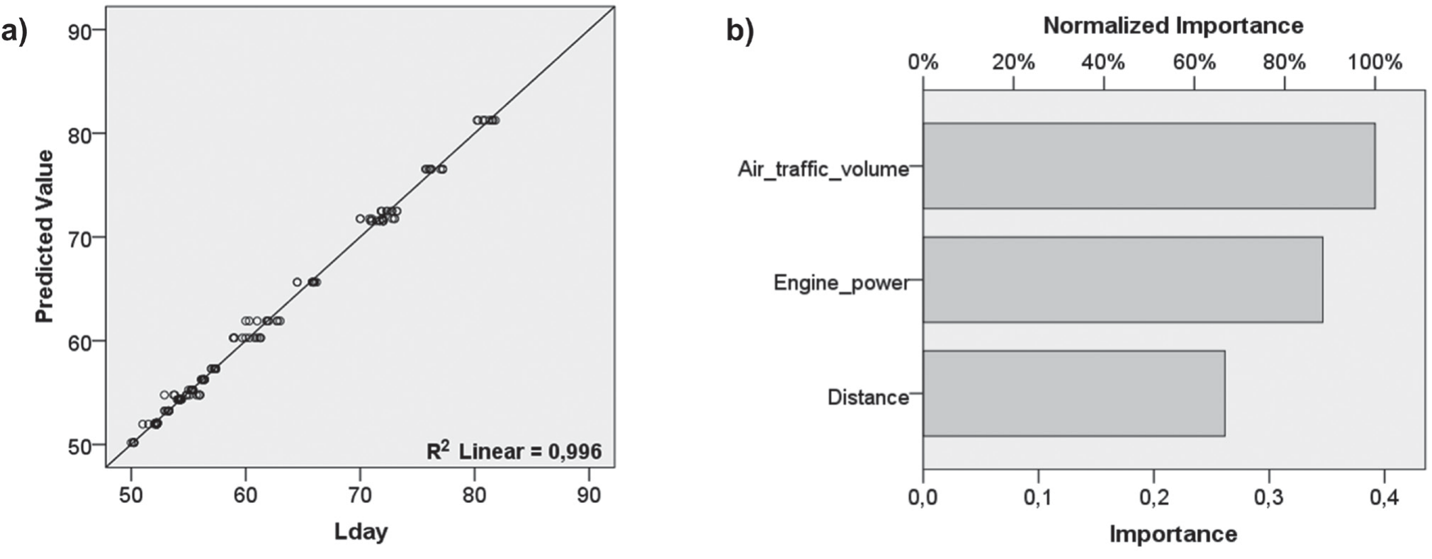
Fig. 6.
Graphic representation of a) actual compared to predicted Levening emission values and b) importance analysis.
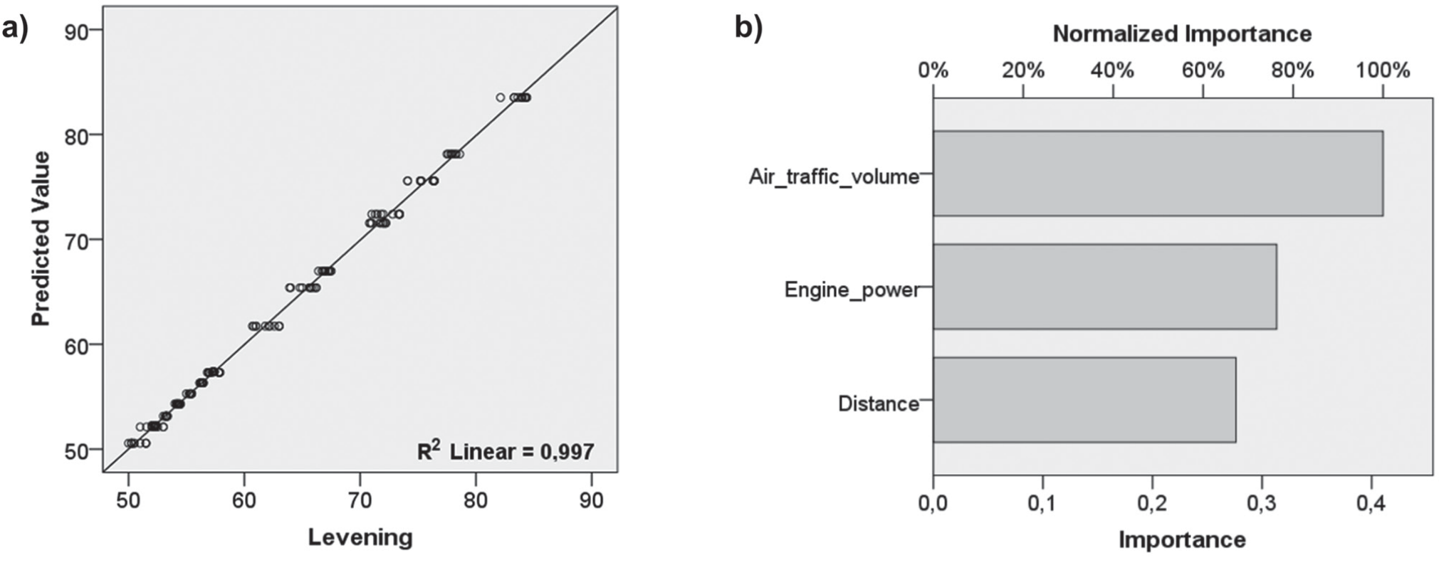
Fig. 7.
Graphic representation of a) actual compared to predicted Lnight emission values and b) importance analysis.
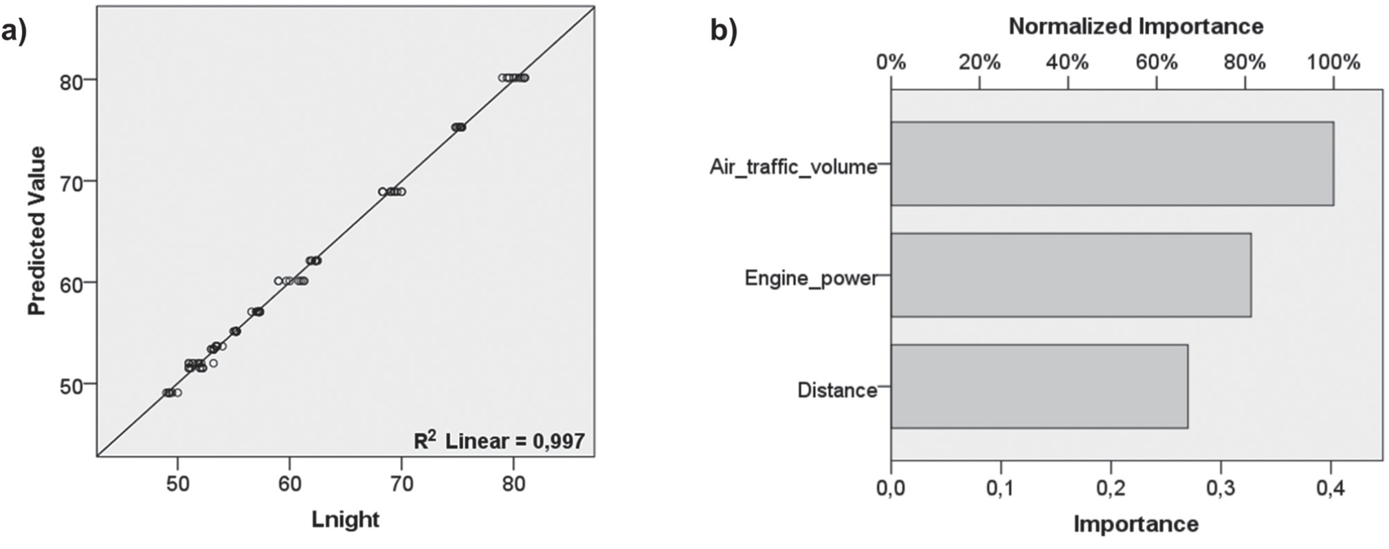
Fig. 8.
Graphic representation of a) actual compared to predicted Lden emission values and b) importance analysis.
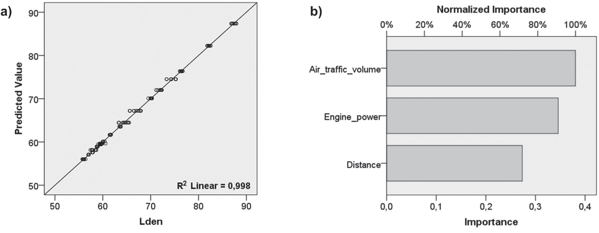
Table 5.
The results of Multiple Linear Regression Analysis.
If we take into consideration the results of the conducted ANN analysis and MLR (the values of R2 and RMSE) it can be concluded that ANN model used in the research offers better results, as Yusof et al. [50] and Kuznetsov et al. [16] also stated in their research.
Conclusions
The results of IDW interpolation method in GIS showed that before the introduction of measures to reduce noise levels caused by air traffic on some grids it was necessary to reduce noise levels by over 30%, while the introduction of measures reduced noise levels, but still on some grids a reduction of over 9% is needed. However, it can be concluded that the application of measures to reduce noise levels in the study area has been successful, but not sufficiently to reach a noise level below the limit values and therefore additional measures to reduce noise should be introduced.
The application of ANNs in the prediction of noise variations has shown that the MLP technique can be successfully used in achieving this goal. The results of this analysis can also be used in the implementation of adequate measures to reduce noise levels. The reliability of the ANNs in predicting noise pollution caused by air traffic was confirmed by higher coefficients of determination and lower RMSE values than the ones achieved by MLR method. However, it is important to point out that additional parameters (the speed of the aircraft during takeoff and landing, wind direction, etc.) may also be included in the analysis, which would probably affect the result of the analysis using MLP technique, or some other traditional model such MLR, but in this way, data would certainly be obtained that would facilitate decision-making on the choice of corrective measures.
Since the research the research was limited both by time and technical possibilities to perform measurements at more measuring points, in future research, within the project carried out by the airport authorities, it is planned that the measuring points are located in the direction of the extended runway, where the highest measured noise values will certainly be. This will certainly make the noise distribution different. Also, it is planned to measure noise east and west of the airport in the vicinity of residential areas, to study the impact of noise on the population living in the vicinity of the airport.
Finally, the system of preferential runways can be introduced in the future. This would make it possible to schedule the use of the runways according to the time of day, as well as according to the days of the week, which would achieve an additional reduction of the noise level in certain periods. It is also possible to introduce a flight ban for aircraft that are not noise certified for night flights. However, these are suggestions for further research.