

Introduction
Carbon dioxide is one of the main greenhouse gases. In 2022, the global CO2 emissions of the transportation industry reached 7.95 Gt, among which the proportion of road transportation was 74%, with substantial potential for carbon reduction [1]. Mountainous plateau areas exhibit relatively high ecosystem vulnerability and are frequently affected by climate change [2, 3]. With economic and societal development, the number of motor vehicles in use will continue to grow. In the Stated Policies Scenario, electric vehicles will account for > 10% of the road vehicle fleet by 2030 [4]. Although the process of vehicle electrification is gradually accelerating, fuel vehicles will still dominate in the coming period. Vehicle CO2 emissions exacerbate the greenhouse effect and have a profound impact on the ecosystem in mountainous plateau areas [5]. Investigating the influencing characteristics of CO2 emissions from vehicles on expressways in mountainous plateau areas and constructing a localized CO2 prediction model are conducive to the effective accounting and control of CO2 emissions.
Mountainous plateau areas have complex topographies and harsh climatic conditions. The impact of the vehicle operating environment and the road alignment on CO2 emissions is more prominent compared to that in low-altitude areas. Real driving emission (RDE) tests indicate that the CO2 emission rates nearly triple when the altitude increases from 2,000 to 4,500 m [6]. Some studies suggest that there is no unified pattern between altitude and CO2 emissions in RDE tests [7]. Although RDE tests provide a more accurate representation of actual emission levels than indoor tests, they introduce additional variables during the testing process, which add greater uncertainty to analyses of CO2 emissions relative to altitude changes. The changes in temperature and humidity along a highway have a significant impact on vehicle CO2 emissions; CO2 emissions significantly increase at high and low ambient temperatures [8, 9]. Real-vehicle tests and indoor simulation tests indicate that at an ambient temperature of -20℃, the CO2 concentration of vehicle emissions at an idle state exceeds 16% [10]. When the relative humidity increases from 10 to 40%, the CO2 emission rate of the light-duty vehicle (LDV) decreases from 4.2 to 3.6 g/s [6]. Furthermore, road alignment indicators substantially influence vehicle CO2 emissions. Dong et al. [11], through real-vehicle tests, concluded that the minimum radius of circular curves affecting vehicle carbon emissions was 500 m. A strong correlation exists between the road grade and carbon emissions [12], whereby carbon emissions increase significantly when the road grade exceeds 3% [13]. On a 3-km section with a slope, where the driving speed of a vehicle decreases by > 20 km/h, fuel consumption is 5-fold greater than when the speed decreases by ≤10 km/h [14]. Moreover, the design of vertical curves on highways significantly affects vehicle carbon emissions. The design of vertical curves with gentle curvatures provides environmental and economic benefits for the entire lifespan of a highway [15]. Currently, research on the impact characteristics of road alignment conditions on vehicle CO2 emissions has focused on grade. However, horizontal alignment is the basis for determining the vehicle operating speed. The continuity of horizontal alignment is equally important for vehicle CO2 emissions, with a lack of research on this topic.
The results of RDE tests are generally higher than the indoor test values under the international LDV emission test cycles and the calculated values by CO2 emission models (such as MOVES and COPERT). Some studies have carried out research on CO2 emission prediction models based on RDE test data. Vehicle CO2 emissions are a multifaceted issue influenced by alignment conditions, environmental characteristics, and operating states. Traditional multiple linear regression analysis cannot reflect the complex nonlinear relationship between emissions and various factors [16]. Some studies have improved the accuracy and interpretability of predictions by constructing machine learning models for vehicle instantaneous emissions [6, 17, 18]. However, the adaptability of the existing machine learning models is limited by the quality and representativeness of the test data. In the mountainous plateau areas, the operating environment of vehicles is complex and changeable, with prominent differential characteristics varying with altitude and seasons. Additionally, within the same altitude range, there are significant differences in road alignment conditions, which are restricted by topographic and geological conditions. Therefore, the model construction based on the real-vehicle emission test data is undoubtedly a few-shot problem, and it requires higher generalization ability and stability of the model.
This study aims to conduct real-vehicle emission tests of LDVs in mountainous plateau areas, analyze CO2 emissions from LDVs, and construct a localized CO2 emission prediction model based on the model-agnostic meta-learning (MAML) algorithm. Our research contributes to the design, planning, and management of expressways in mountainous plateau areas as follows.
1) Due to the steep terrain in the mountainous plateau areas, vehicles show notable differences in engine load and operating conditions between the upslope and downslope directions, and the influencing characteristics of CO2 emissions vary accordingly. We quantify the influence of various factors on CO2 emissions from LDVs when driving upslope and downslope using the built-in feature importance and partial dependence of random forest (RF), and analyze the variation law of CO2 emissions with different influencing factors;
2) The road alignment determines the operating state of vehicles. By analyzing the distribution patterns and variation trends of vehicle CO2 emissions under different horizontal and vertical alignment conditions, data support can be provided for the low-carbon alignment design of expressways in mountainous plateau areas;
3) We explore the variation law of CO2 emissions from LDVs in the same Vehicle-specific power (VSP) interval with the increase of altitude, and analyze the characteristics of vehicle CO2 emissions in response to the changes in operating environment; 4) We improve the generalization of the CO2 emission prediction model in unknown altitude scenarios and realize effective predictions of CO2 emissions for LDVs on mountainous plateau expressways by adopting a few-shot learning strategy and constructing a regression model based on the MAML algorithm. This study contributes to addressing knowledge gaps in CO2 emissions from LDVs traveling on expressways in mountainous plateau areas, specifically considering upslope and downslope driving, road horizontal alignment, and altitude. The study findings can be applied to the formulation of CO2 emission management policies for highway transportation and the optimization of low-carbon road engineering in mountainous plateau areas, providing fundamental support for the development of low-carbon transportation on expressways in mountainous plateau areas.
Materials and Methods
Test Instrumentation
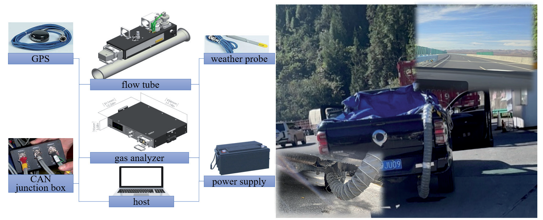
Real-vehicle tests were conducted using a portable emission measurement system (PEMS). The test instrument was a SEMTECH Fuel Economy Meter, which included components such as a flow tube, gas analyzer, global positioning system (GPS), power supply, and weather probe (Fig. 1). The flow tube primarily employed a Pitot tube based on Bernoulli’s principle to calculate the mass flow rate by measuring the pressure difference in the gas flow. The gas analyzer utilized nondispersive infrared technology to analyze dried and filtered samples and measure CO and CO2 concentrations in exhaust gas.
Data obtained from the test consisted of the exhaust emission rate, CO2 concentration, exhaust temperature, GPS three-dimensional coordinates, instantaneous speed, acceleration, atmospheric pressure, ambient temperature, and relative humidity. The test cycle lasted for 1 s.
Data Processing
Alignment Conditions
ACR represents the change in the deflection angle (°) per unit length (m) traveled by the vehicle within each second. The change in the unit deflection angle was calculated based on the difference in the azimuth angles during adjacent periods:
where ACRi is the deflection angle change rate at the i-th second (°/m), azii~i+1 is the azimuth angle from the i-th second to the (i + 1)-th second (°), and vi is the vehicle speed at the i-th second (m/s).
In this study, t was calculated based on the mileage traveled by the vehicle per second and the altitude difference:
where t is the vertical rise/slope length and alti is the altitude at the i-th second (m).
Operating States
VSP represents the instantaneous output power of a vehicle when moving one unit of mass, which was computed based on Equations (3)-(6) [19]:
where m is vehicle mass (t), s is time (s), a is vehicle acceleration (m/s2), εi is the mass factor, g is the acceleration of gravity (m/s2), CR is the coefficient of rolling resistance, CD is the drag coefficient, A is the frontal area of the vehicle (m2), ρa is the ambient air density (kg/m3), vW is the headwind into the vehicle (m/s), H is vehicle height (m), hg is ground clearance (m), W is vehicle width (m), P is standard atmospheric pressure (kPa), P1 is atmospheric pressure (kPa), and T1 is ambient temperature (K).
Based on the total mass of the test vehicle, its external dimensions, and the relevant technical parameters, a formula for the VSP of the test vehicle was derived:
CO2 Emissions Rate
Using data on the exhaust emission rate, temperature, CO2 wet concentration, and atmospheric pressure, the CO2 emission rate was calculated as follows [20]:
where φCO2wct is the CO2 wet concentration (%), φCO2dry is the CO2 dry concentration (%), kW is the dry–wet correction factor, λ is the H molar ratio, Ha is the absolute humidity of the intake air (H2O/dry air) (g/kg), RH is the relative humidity (%), and Ps is the saturation vapor pressure (kPa). We then obtained the following:
where ERCO2 is the CO2 emission rate (g/s), EER is the exhaust emission rate (L/s), ρCO2 is the CO2 density (g/L), P2 is the exhaust pressure (Pa), M is the molar mass (mol), R is the gas constant (8,314 Pa/[mol·K]), and T2 is the exhaust temperature (K).
Test Route
A 288-km expressway section in the mountainous areas of the western Sichuan Plateau was selected as the real-vehicle emission test route, including the Ande‒Zhe Gu Mount section of the Chengdu‒Changdu Expressway G4217, and the Shuanjinsi‒Rangkou and Aba‒Jiuzhi sections of the Jiuzhi‒Barkam Expressway G0615 (Fig. 2).
Fig. 2.
Test route and distribution of a) altitude, b) angle change rate, and c) grade. ACR: angle change rate; t: road grade.
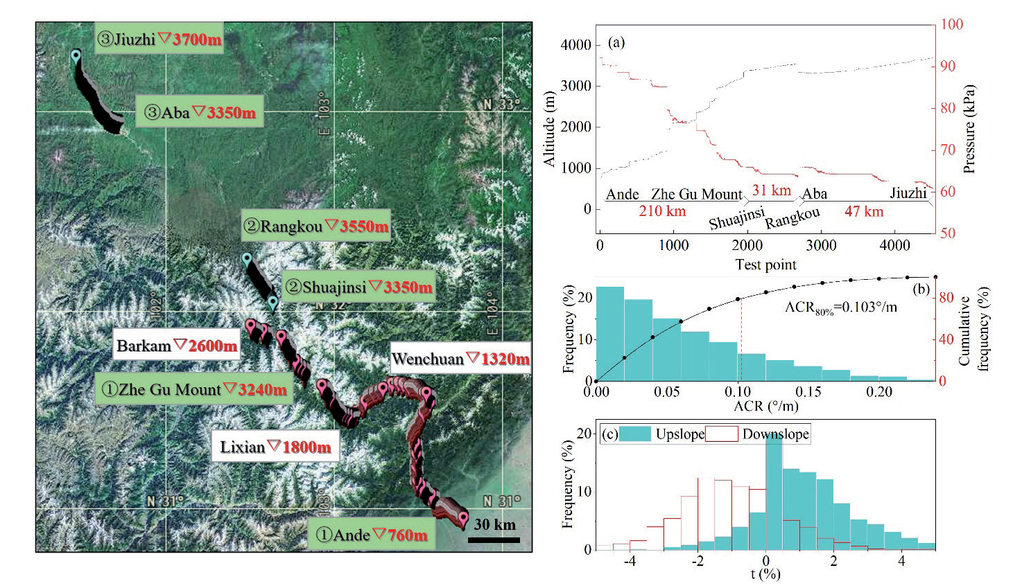
Fig. 2a) shows that the altitude of the Ande‒Zhe Gu Mount section increases from 760 to 3,240 m, that of the Shuanjinsi‒Rangkog section increases from 3,350 to 3,550 m, and that of the Aba‒Jiuzhi section increases from 3,350 to 3,700 m. Fig. 2b) indicates that the ACR distribution exhibited a decreasing trend, with the 80th percentile at 0.103 °/m. Fig. 2c) shows that the interquartile range of the grade in the upslope direction from Ande to Jiuzhi was (0.37%, 1.97%), and the interquartile range of the grade in the downslope direction from Jiuzhi to Ande was (-1.89%, 0%). The real-vehicle test used sections of open roads as the research object and excluded tunnel sections. A total of 9,381 datasets were collected, of which 4,513 sets were in the upslope direction from Ande to Jiuzhi and 4,868 sets were in the downslope direction from Jiuzhi to Ande.
Test Vehicles
A light gasoline pick-up truck was used in the real-vehicle emission tests. During the test period, all fuel for the vehicle was sourced from the same gas station. Moreover, the same local driver operated identical CO2 emission testing instruments to complete the tests from March 10-12, 2024. Detailed parameters of the test vehicle are provided in Table 1.
Model Evaluation Indicators
The accuracy of the CO2 emissions prediction model was evaluated using the mean squared error (MSE), root mean squared error (RMSE), and mean absolute error (MAE). MSE is the mean value of the squares of the differences between the predicted and actual values:
where N is the sample size, Yi is the actual value, and Ŷi is the predicted value. RMSE is the square root of the MSE, calculated as follows:
MAE is the mean value of the absolute errors between the predicted and actual values, calculated as follows:
Results and Discussion
Factors Influencing CO2 Emissions
The main factors influencing the CO2 emissions of vehicles on expressways in mountainous plateau areas included the VSP, speed, acceleration, altitude, atmospheric pressure, air density, temperature, humidity, grade, and ACR. Among these factors, differences in the altitude and ACR may have led to variations in environmental conditions and vehicle operating states, thereby further affecting vehicular CO2 emissions. This study analyzed the characteristics influencing each factor for the vehicle CO2 emission rate from direct and indirect perspectives.
Direct Factors
When the vehicle was driven in the downslope direction, the slope component of the gravitational force performed positive work, and there were more idle driving conditions than when the vehicle was driven in the upslope direction. The influence of the various factors on CO2 emissions differed. Therefore, based on vehicle CO2 emission data in the Ande‒Jiuzhi and Jiuzhi‒Ande directions, RF models were constructed to analyze the influence of various factors when the vehicle was driving in the upslope and downslope directions.
The adopted RF algorithm comprised decision trees and a bagging algorithm, based on various independent tree-shaped classifiers [21]. Each decision tree was trained using randomly selected subsamples and features to ensure high model diversity. The main model parameters included the number of estimators, maximum depth, minimum sample split, minimum sample leaf, and maximum features of the decision trees (Fig. 3).
The built-in feature importance in an RF is a measure for evaluating the degree of influence of the features on the prediction results [22]. This study utilized built-in feature importance to quantify the degree of influence of each influencing factor on the target feature CO2 emission rate (Fig. 4). A comparative analysis was then conducted on the differences in feature importance for each influencing factor in the upslope and downslope directions.
Table 1.
Vehicle parameters.
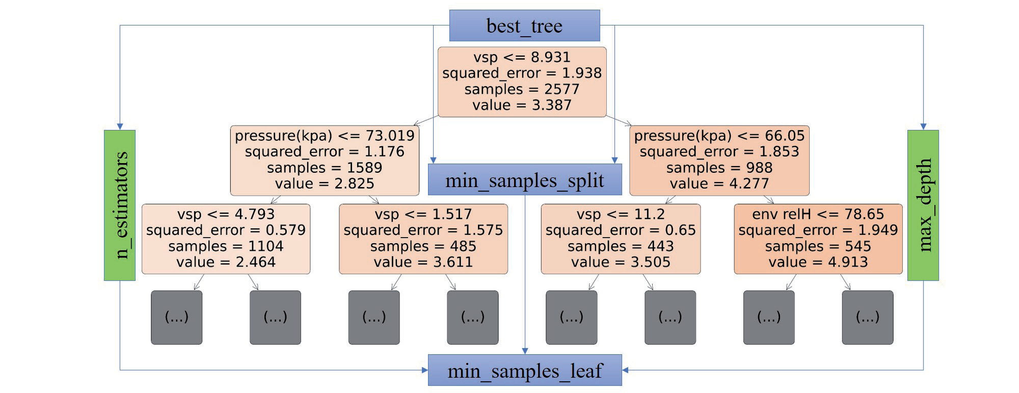
Fig. 4 shows that when the vehicle was driving in the upslope and downslope directions, the top three factors ranked in descending order of feature importance were VSP > air density > atmospheric pressure. The feature importance of VSP in the upslope and downslope directions was 0.25 and 0.22, respectively, and those of air density and atmospheric pressure were approximately 60% of that of the VSP. Using the standard deviation method, importance was divided into high-, medium-, and low-importance groups according to the ranges (0, X̅ -S), (X̅ -S, X̅ +S), and (X̅ +S,1), respectively (Table 2). Among them, VSP was the only factor in the high-importance group, which was the most important factor in determining the CO2 emission rate of the LDV in mountainous plateau areas.
When the vehicle was driving in the downslope direction, the feature importance of the grade was 9% lower than that when the vehicle was driving in the upslope direction. The influence of the grade on the CO2 emission rate not only involved changes in the operating state of the engine, but was also reflected in vehicle speed variations at different grades. When driving downslope, the vehicle operating speed could be more easily maintained at the expected level, the speed distribution was more concentrated, and moving downslope was advantageous for the engine load. Therefore, the degree of influence of the grade was lower in the downslope direction than in the upslope direction.
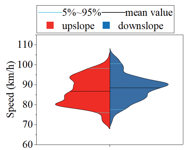
Additionally, when the vehicle was driving in the upslope direction, the factor exhibiting the largest change rate in feature importance compared with the downslope direction was speed, which decreased by approximately 43%. This was primarily related to differences in the vehicle operating states in the upslope and downslope directions (Fig. 5). The speed distribution of the vehicles in the upslope direction was more dispersed than that in the downslope direction. When the vehicle was driving in the upslope direction, the percentage of speeds > 80 km/h decreased by 11% compared to that when the vehicle was driving in the downslope direction, resulting in a lower proportion of high-speed operating conditions; consequently, the influence of speed on the CO2 emission rate decreased.
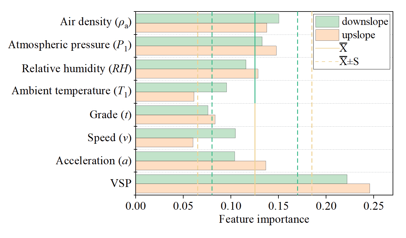
Table 2.
Feature importance grouping
| Group | Low-Importance | Medium-Importance | High-Importance |
|---|---|---|---|
| Downslope | t | ρa, P1, RH, T1, v, a | VSP |
| Upslope | T1, v | ρa, P1, RH, a, t | VSP |
Partial dependence characterizes the overall influence of each factor on the prediction results of the model when the values of the other features are averaged. By fixing the other features, the predicted values of all samples were computed under a series of values for a certain feature. The average of the predicted values was used to obtain the corresponding partial dependence values [23]. Fig. 6 shows the partial dependence curves for each influencing factor.
Fig. 6 shows that the partial dependence values of each factor when the vehicle was traveling in the upslope direction were greater than those when the vehicle was driving in the downslope direction. The partial dependence curves for acceleration, air density, relative humidity, atmospheric pressure, grade, and VSP in the upslope and downslope directions were similar. Among them, the partial dependence curve for acceleration displayed an “S shape”. The CO2 emission rates of the vehicle under different operating conditions increased from deceleration < uniform speed < acceleration, with a maximum difference of 0.9 g/s in the CO2 emission rate under acceleration and deceleration conditions. Additionally, the partial dependence curve for the relative humidity exhibited a stair-step increasing trend. A high-humidity environment is likely to affect the working efficiency of an engine, with critical humidity levels for the main steps in the upslope and downslope directions of 40 and 60%, respectively. Partial dependence curves for the grade and VSP showed nonlinear increasing trends, with maximum differences in partial dependence values for the upslope direction of 0.33 and 1.43 g/s, respectively, and 0.34 and 1.28 g/s, respectively, for the downslope direction.
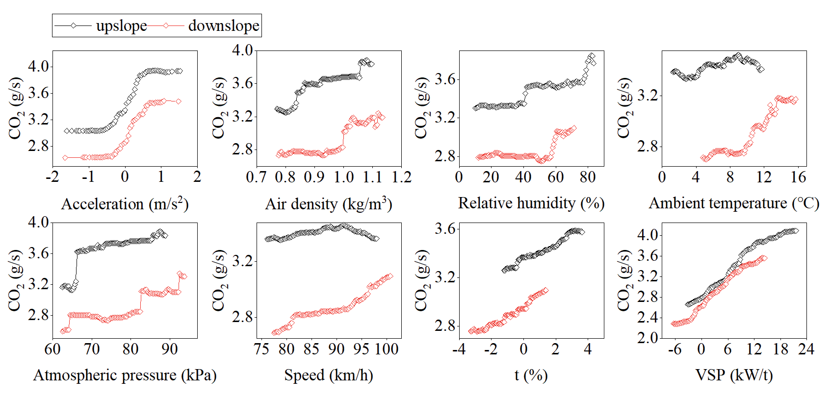
There was a significant difference in the partial dependence curves of temperature and speed when the vehicle was driving in the upslope and downslope directions. When driving in the downslope direction, the variation in the amplitude of the CO2 emission rate with increasing temperature and speed was greater than that when the vehicle was driving in the upslope direction. The CO2 emission rate increased by 0.5 g/s when the temperature in the downslope direction increased from 4.8 to 15.7°C. However, the maximum difference in the CO2 emission rate was only 0.1 g/s when the temperature in the upslope direction increased from 1.3 to 11.7°C. Additionally, the CO2 emission rate was the lowest when the minimum speed in the downslope direction was 77 km/h, similar to the economical vehicle speed. The maximum difference in the CO2 emission rate was 0.4 g/s. The CO2 emission rate in the upslope direction showed a single-peak curve with an increase in speed, reaching its peak at 92 km/h; however, the maximum difference in the CO2 emission rate was only 0.1 g/s.
Indirect Factors
The per-second ACR reflects the vehicle operating states under different horizontal alignment conditions and is related to the vehicle driving speed and deflection angles of horizontal curves. Grade intervals were categorized based on t < -1%, -1% ≤ t < 1%, and t ≥ 1%. Similarly, ACR intervals were defined as ACR < 0.0143 °/m, 0.0143 °/m ≤ ACR < 0.0286 °/m, 0.0286 °/m ≤ ACR < 0.0409 °/m, 0.0409 °/m ≤ ACR < 0.0716 °/m, and ACR ≥ 0.0716 °/m. This analysis focused on the distribution patterns of vehicle CO2 emission rates within different grades and ACR intervals, as well as the variations in their mean distributions with the ACR (Figs. 7 and 8).
Fig. 7 shows that the distribution patterns of the CO2 emission rates at different grades and ACR intervals exhibited a single-peak shape, with their 25-75% quantile intervals primarily located on the right side of the peak. The distribution pattern was similar to a Gamma distribution, with all p-values for the distribution fitting > 0.01; notably, 67% of the intervals had a p-value > 0.05. The probability density function is given as follows:
Fig. 7.
Distribution pattern of CO2 emission rates in different grade and angle change rate intervals. P*: statistical significance (p-value); IQR: interquartile range; α: shape parameter; β: inverse scale parameter; t: road grade; ACR: angle change rate.
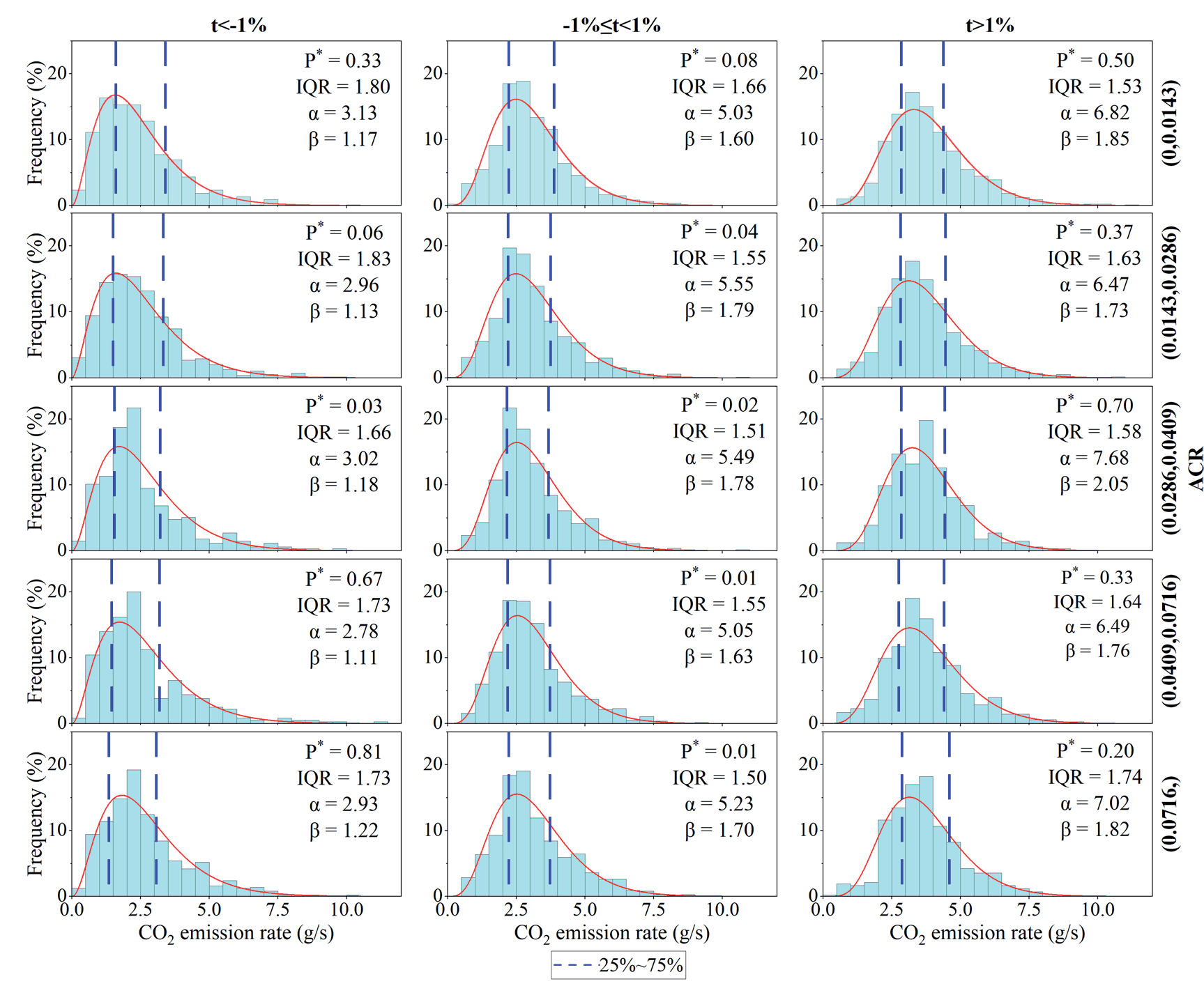
Fig. 8.
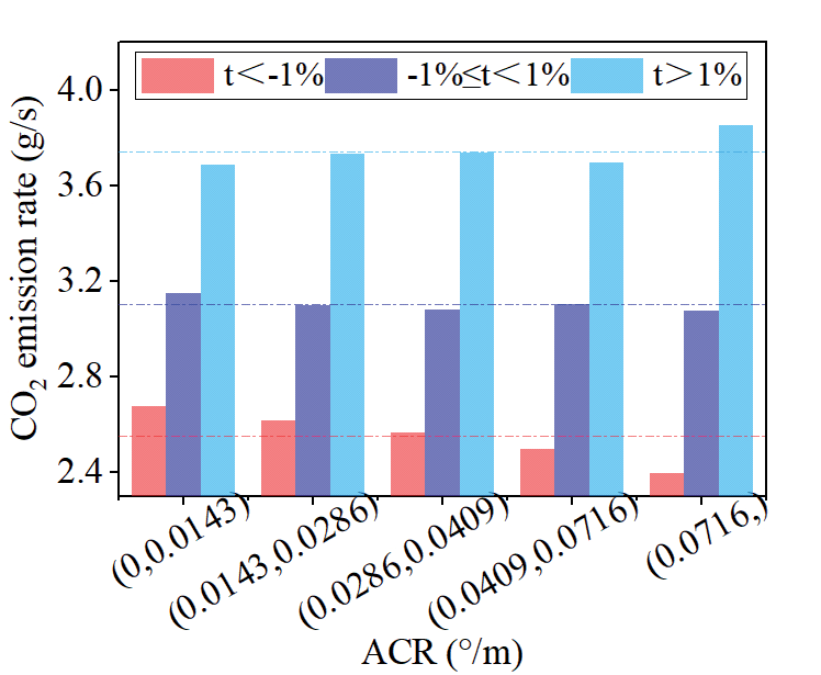
Distribution mean of CO2 emission rates in different grade and angle change rate intervals. t: road grade; ACR: angle change rate.
where α is the shape parameter, β is the inverse scale parameter, and Г(α) is the Gamma function. In the same ACR interval, when t ≥ 1%, the α and β values of the CO2 emission rate distribution were larger than those when t < -1%. This resulted in a more symmetrical distribution pattern, with a shorter tail, a rightward shift in the distribution centre, and an increased distribution concentration.
Fig. 8 shows that the mean CO2 emission rate distribution within the same ACR interval increased with an increase in grade intervals. When ACR > 0.0716 °/m, the difference in the mean CO2 emission rate distribution between t ≥ 1% and t < -1% was the largest, with a maximum difference of 1.5 g/s.
Furthermore, variation trends in the mean CO2 emission rate distribution within the different grade interval differed with increasing ACR intervals. When t < -1%, the mean vehicle CO2 emission rate distribution exhibited an overall decreasing trend with increasing ACR, with a range of 0.28 g/s. When -1% ≤ t < 1%, the mean vehicle CO2 emission rate distribution fluctuated slightly as ACR increased, with a range of 0.07 g/s. When t ≥ 1%, the mean vehicle CO2 emission rate distribution showed an overall increasing trend with increasing ACR, with a range of 0.17 g/s. This may have been because the importance of acceleration in the upslope sections was higher than that of speed. The initial speed of the vehicle entering the curved unit was relatively low, and the acceleration gradient upon exiting the curved unit increased as the radius decreased, leading to a corresponding increase in the CO2 emission rates. In contrast, in downslope sections, the importance of speed slightly outweighed that of acceleration. The initial speed of the vehicle entering the curve unit was relatively high; the smaller the radius, the lower the vehicle operating speed, such that it was closer to the economical vehicle speed, resulting in a decrease in the CO2 emission rates.
There were differences in the air density, atmospheric pressure, ambient temperature, and relative humidity across different altitude ranges, all of which had significant effects on vehicular CO2 emissions. Air density and atmospheric pressure decreased as altitude increased, and the air resistance acting on the vehicle diminished; however, the engine air:fuel ratio decreased, resulting in reduced vehicle power performance. Additionally, temperature and humidity fluctuations may have influenced the heat released during fuel combustion. These factors collectively contributed to variations in the vehicle CO2 emissions.
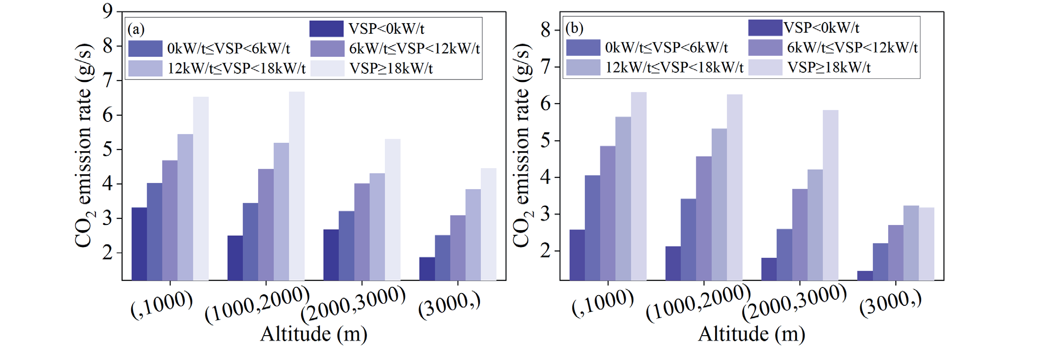
VSP intervals were classified as follows: VSP < 0 kW/t, 0 kW/t ≤ VSP < 6 kW/t, 6 kW/t ≤ VSP < 12 kW/t, 12 kW/t ≤ VSP < 18 kW/t, and VSP ≥ 18 kW/t. This analysis aimed to examine the trends in the CO2 emission rates for vehicles within the same VSP interval on the upslope and downslope sections with changes in altitude (Fig. 9).
Fig. 9 shows that within the same VSP interval, the CO2 emission rate decreased as the altitude increased, and the reduction amplitude of the CO2 emission rate became more pronounced with an increasing VSP. When VSP ≥ 18 kW/t and the altitude increased from < 1,000 to > 3,000 m, the CO2 emission rates on the upslope and downslope sections decreased by 32 and 50%, respectively.
Real-vehicle tests conducted in the altitude simulation chamber indicated that when the temperature and humidity were set at 25ºC and 40%, respectively, during the high-speed operation phase of the WLTC for a naturally aspirated test vehicle, the CO2 emission factor decreased by 13.5% when the altitude increased from 0 to 2,500 m [24]. This reduction was mainly due to decreased air resistance; however, the reduction in the air:fuel ratio was more likely to lead to an increase in the CO2 emissions. In this RDE test on the expressway in mountainous plateau areas, the ambient temperature and humidity of the test section exhibited significant changes with increased altitude (Fig. 10).
Fig. 10 shows that the overall mean ambient temperature and relative humidity exhibited decreasing trends with an increase in altitude. The temperature and relative humidity distribution intervals on the upslope and downslope sections were essentially the same, with a temperature distribution interval of (4°C, 16°C) and a humidity distribution interval of (20%, 80%). Within the same VSP interval, ambient temperature and relative humidity were among the primary factors influencing the CO2 emissions of vehicles on expressways in mountainous plateau areas. Furthermore, within the temperature and humidity distribution ranges of the test section, a lower ambient temperature and humidity corresponded to lower vehicle CO2 emission rates. Comparative Analysis of CO2 Emission Prediction
Models Based on MAML and RF Algorithms
Traditional learning methods are restricted by the scarcity of data in the analysis of few-shot problems and have difficulty in effectively extracting and representing data features. Consequently, they perform poorly in performance dimensions such as accuracy, generalization ability, and stability of the models. The MAML algorithm is a meta-learning approach that rapidly learns to adapt model parameters through gradient descent. It uses prior knowledge and experience to guide the learning of new tasks, thereby endowing the network with the ability to learn [25]. This method does not introduce learning parameters specific to meta-learning and is compatible with any model trained via gradient descent, making it applicable to few-shot learning problems. The mathematical expression for a single task in the algorithm is expressed as follows:
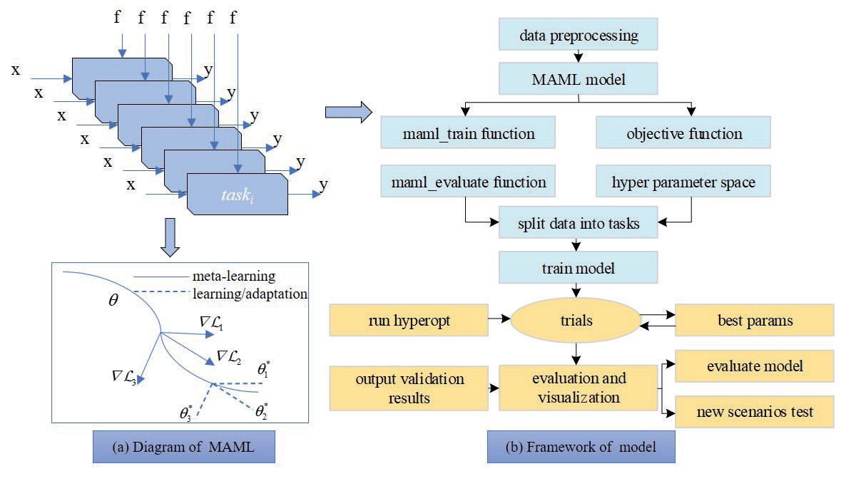
where T is the task, L is the loss function, x is the observations, a is the output, q(x1) is the distribution over initial observations, q(xi+1|xi,ai) is the transition distribution, and H is the episode length. A schematic of the algorithm is presented in Fig. 11a) [26].
Fig. 11a) shows that when adapting to a new task Ti, the model’s parameters θ become θi', calculated as follows:
where ∇L is the gradient descent update, α is the step size, and fθ is the parametrized function. The objective of the MAML algorithm is to determine a set of parameters for θ that have representative capabilities for multiple tasks. The update of θ comprises two stages: the update and optimization for a specific task and optimization of the MAML model.
The MAML algorithm was employed for model training and evaluation to construct a CO2 emissions prediction model based on a neural network model architecture composed of multiple linear layers and a ReLU activation function. Fig. 11b) illustrates the model framework. The main processes included meta-training, in which the MSE loss function, nn.MSELoss, was used to measure the difference between the predicted and actual values. The torch.optim.Adam optimizer was selected to adaptively adjust the learning rate of the parameters. The model was optimized based on the learning rate (alpha) and weight decay (weightdecay), as well as hyperparameter optimization, whereby the hp.loguniform function in the Hyperopt library was used to define the hyperparameter search space. The hyperparameters of the model were optimized by processing the data from multiple tasks and calculating the MSE. A new task testing was implemented when the trained model was utilized to obtain the predicted values on new tasks, and the evaluation metrics (i.e., MSE, MAE, and RMSE) of the model were calculated.
The RF and MAML CO2 emission prediction models were constructed using 8,431 sets of real-vehicle test data within the altitude range from 600-3,550 m as the model training and validation sets. Fig. 12 shows the predicted and actual values of the models in the validation set. The results demonstrated that the correlation between the predicted and actual values of the MAML model on the validation set was superior to that of the RF model, with R2 values of 0.72 and 0.69, respectively.
We used 950 sets of real-vehicle test data within an altitude range of 3,550-3,730 m as the test set for the model in the new scenario. Compared to the training task, the new task operated at a higher altitude, resulting in significant differences in the atmospheric pressure and air density distributions (Fig. 13). Fig. 14 presents the evaluation metrics of the model on the validation and test sets.
Fig. 10.
Variation curve of ambient temperature and relative humidity with altitude from a) t ≥ 0% and b) t < 0%. VSP: vehicle-specific power; t: road grade.
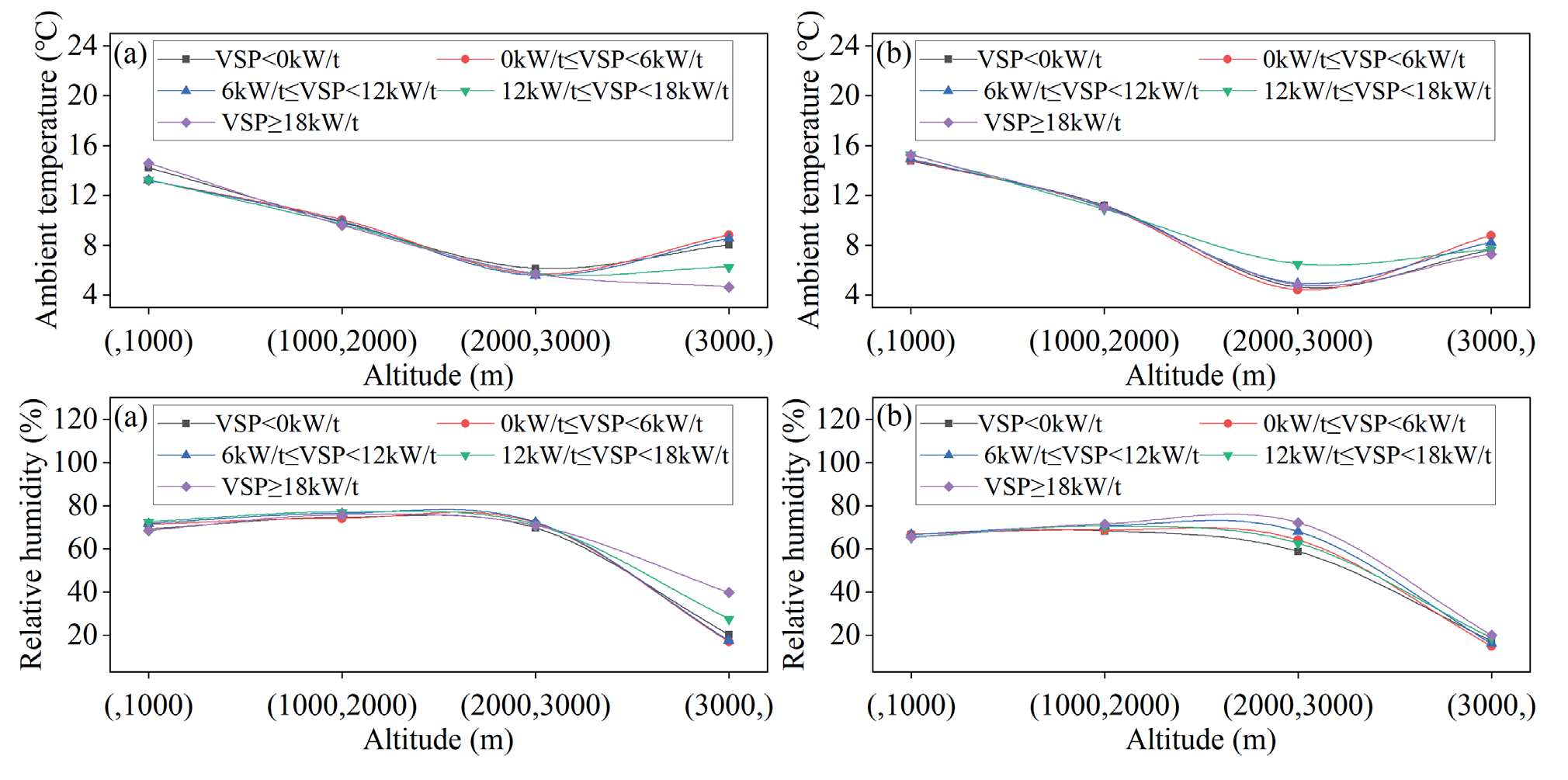
Fig. 11.
Structure of the model-agnostic meta-learning model. θ: the model’s parameters; ∇L: gradient descent updates; MAML: modelagnostic meta-learning.
Although the pressure and air density distributions of the new task contained data that were not observed or were only minimally covered during training, the predicted total CO2 emissions on the test set from the RF and MAML models were 2,333 and 2,327 g, respectively, both of which reached 99% of the actual total CO2 emissions. The constructed CO2 emission prediction model demonstrated high precision and could be utilized for the calculation and management of the total CO2 emissions of the LDV on expressways in mountainous plateau areas.
Fig. 12.
Comparison between predictions and true values. RF: random forest; MAML: model-agnostic meta-learning.
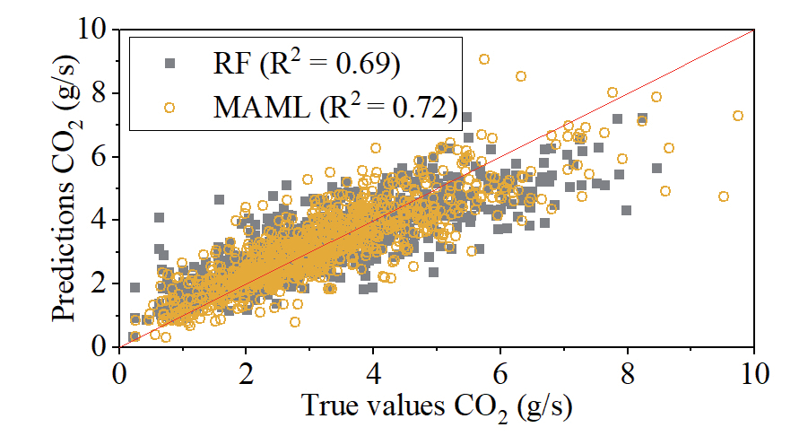
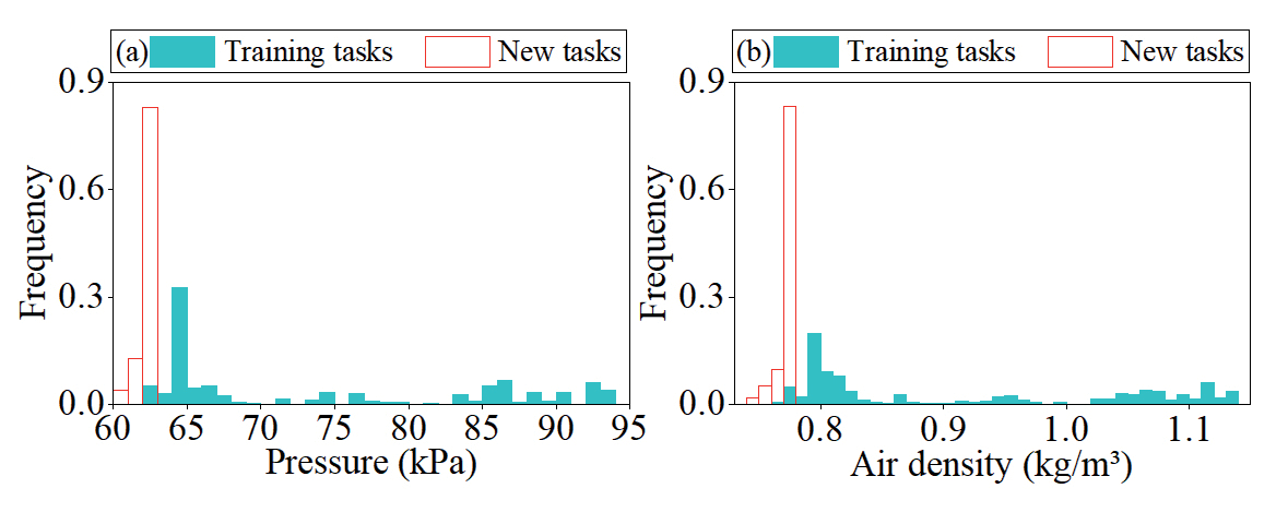
Fig. 14.
Evaluation metrics of random forest (RF) and model-agnostic meta-learning (MAML) models on validation (Val) and test sets. MSE: mean squared error; RMSE: root mean squared error; MAE: mean absolute error.
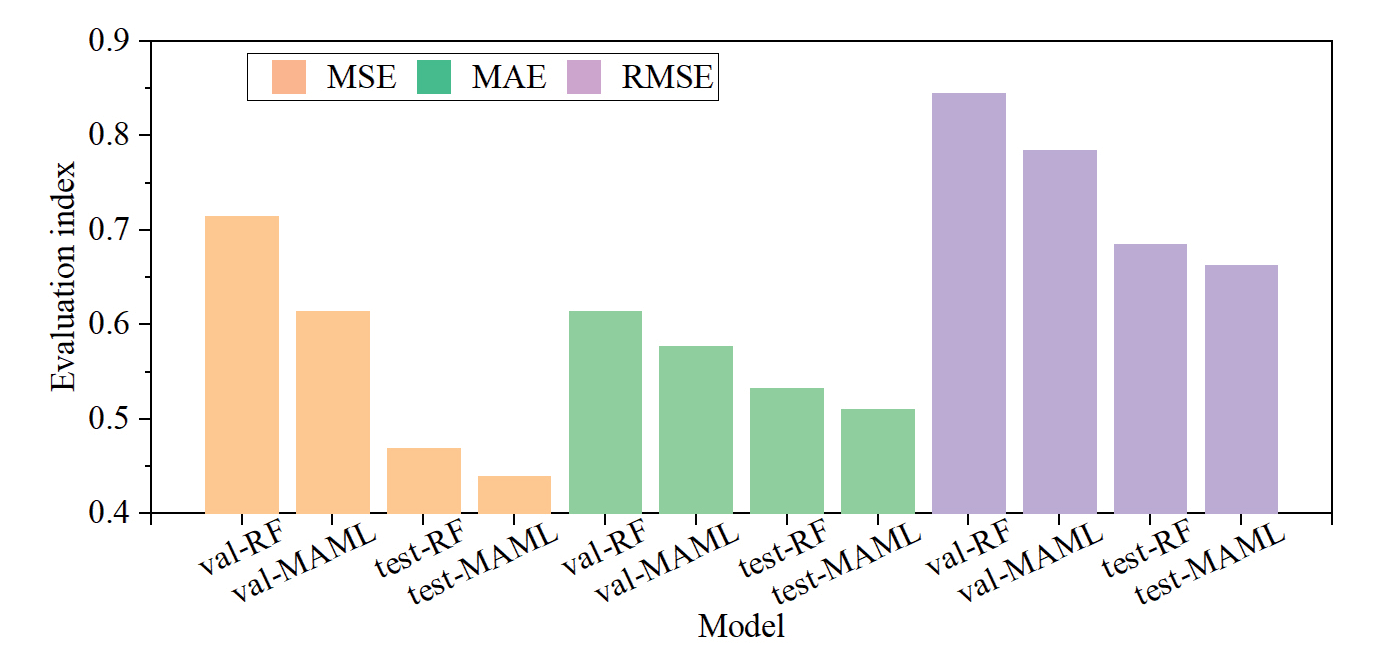
Furthermore, the MSE, MAE, and RMSE evaluation metrics of the MAML model on the validation and test sets outperformed those of the RF model. Specifically, the MSE, MAE, and RMSE for the validation set were reduced by 14, 6, and 7%, respectively; whereas, those for the test set were reduced by 6, 4, and 3%, respectively. The RF model was more limited to the training and prediction of the current task, whereas the generalization ability of the MAML model was superior, resulting in a higher adaptability to unknown tasks.
Conclusions
This study conducted CO2 emission tests of LDV on expressways in the western Sichuan Plateau mountainous areas using a PEMS, leading to the following conclusions.
First, the results of the feature importance analysis based on the RF model exhibited significant differences between the upslope and downslope directions. Speed had the greatest importance change, decreasing by approximately 43% from the downslope to the upslope directions. The feature importance of VSP in the upslope and downslope directions was 0.25 and 0.22, respectively. VSP was the most critical factor determining the CO2 emission rate compared with the environmental and road-related factors in the mountainous plateau areas. Second, the variations in the mean CO2 emission rate distribution within the different grade interval differed with increasing ACR intervals. In the intervals of t < -1%, -1% ≤ t < 1%, and t ≥ 1%, the trends were decreasing, stable, and increasing, respectively, with ranges of 0.28, 0.07, and 0.17 g/s, respectively. This indicates that the steeper the grade, the more notable the influence of ACR on the CO2 emission rate. Third, the mean CO2 emission rate within the same VSP interval decreased as the altitude increased, which was associated with the temperature and humidity distribution characteristics along the test section. The amplitude of this decrease became more pronounced with an increasing VSP. Finally, the MAML model demonstrated a significantly enhanced generalization capability for unknown tasks compared to the RF model, as evidenced by its superior performance in predicting CO2 emission rates, with MSE, MAE, and RMSE values decreasing by 6, 4, and 3%, respectively. The model can be effectively applied to the accounting and assessment of CO2 emissions during both highway design and operational phases.
In terms of research prospects, this study was limited to an examination of the CO2 emission characteristics of LDVs. In the future, tests and analyses of other types of vehicles can be supplemented to enrich the accounting methods and management strategies for the CO2 emissions of vehicles on mountainous plateau expressways.