

Introduction
With the acceleration of urbanization, the problem of urban air pollution is becoming increasingly prominent [1, 2]. Air pollution not only causes serious damage to the urban ecological environment, but also poses a threat to the health of urban residents [3, 4]. Healthy urban space (HUS) refers to the creation of urban spaces that are conducive to the health of residents, taking into account multiple values such as environment, society, economy, and health in urban planning and construction. In a HUS, the prediction of urban air pollutant concentration and optimization of health risk assessment have become important research directions.
UAPCP is a regression task, and the input data is a time series. To solve this type of time series prediction problem, engineers, scholars, and professors in the industry have conducted extensive research [5, 6]. Lin et al. proposed a new multi-step prediction method for the thermal parameters of ultra-high voltage transformers with LSTM time series networks and conditional mutual information. To increase the calculation efficiency and remove redundancy, the feature selection algorithm with conditional mutual information was utilized to analyze the correlation among the original monitoring parameters. This model was used to predict the trend of changes in oil temperature and winding temperature at different positions of ultra-high voltage transformers. The findings denoted that this method’s accuracy was significantly improved in one-step and multi-step thermal parameter prediction, and RMSE and mean absolute error (MAE) were superior to other existing methods. This offered a novel and effective prediction model for the field of time series prediction [7]. Zhou et al. evaluated the accuracy of several classic time series prediction statistical methods. A novel decomposition method was utilized to process specific time series of daily data. By combining four traditional methods, it could lessen RMSE and improve prediction accuracy. The outcomes indicated that the error rate of this method has been reduced by 10% to 20%. The author team proposed a model that used the generation confrontation model and LSTM as the generator to predict the website traffic time series. Comparing the prediction performance of traditional statistical methods, the experimental findings indicated that there was no significant difference between the two schemes for the prediction accuracy of this specific time series [8]. Ajith et al. proposed a novel multimodal fusion network for predicting solar radiation. Because of the intermittent and uncertain nature of solar energy, the collection in the short term posed new challenges, making accurate prediction an important aspect of power system operation and management. Existing models only used time series data for solar radiation prediction, but in cloudy weather, these models could not quickly capture the nonlinear spatiotemporal changes of data in the short term. To compensate for this deficiency, a new multimodal fusion network was proposed in the study, which used infrared images and past solar radiation data for microscopic prediction of solar radiation. This network extracted spatial and temporal information in parallel and used fully connected neural networks for fusion. The experimental outcomes expressed that the multimodal fusion network outperformed existing methods in predicting solar radiation in cloudy and mixed weather conditions, with an accuracy of 99.23%. When making longer-term predictions, the proposed model exhibited the best balance between performance and testing time [9]. Somu et al. proposed a reliable energy demand prediction model for the growth of global building energy demand. This model utilized energy consumption data recorded at predefined intervals to offer accurate predictions of building energy consumption. This model used k-means clustering for clustering analysis to understand energy consumption patterns and trends and used convolutional neural networks to extract complex features and nonlinear interactions. LSTM was applied to handle long-term dependencies. The efficiency and applicability of the model were proven by using real-time building energy consumption data from a four-story building. Comparing this model with the k-means variant of the most advanced energy demand forecasting model, the findings indicated that the accuracy of the traditional model was lower than that of this model [10]. Yang et al. explored the impact of weather on energy forecasting and emphasized the importance of numerical weather forecasting in energy forecasting practices such as load forecasting, renewable energy generation forecasting, and others. It was found that, due to the shortage of historical weather prediction data, there was a certain gap between such prediction models and practical applications. For this reason, the author provided the numerical weather prediction data set from high resolution model. This dataset could support the various energy prediction tasks mentioned above [11]. Ma studied the prediction problem of industrial power consumption. The goal of this study is to simulate and predict industrial power consumption in Jiangsu province through the nonlinear transformation of time variables. Through that, industrial enterprises in Jiangsu can rationally arrange their next electricity requirement and guarantee the smooth progress of industrial activities. The final research outcomes indicated that the time series regression prediction model put forward in the study could well simulate and forecast the findings of industrial power consumption, providing new perspectives and methods for data prediction and time series prediction [12].
Previous studies have shown that traditional prediction methods are mainly based on statistical models, such as regression analysis, time series analysis, etc. Although these methods are simple and easy to use, their ability to handle complex nonlinear relationships and dynamically changing environmental factors is weak. For example, in references [8] and [10], although both used the LSTM algorithm with excellent predictive performance for time series data to construct prediction models, both only improved the prediction accuracy of the data from the perspective of using multiple algorithms to process the data sequentially and improving the algorithm's structure. From the perspective of test results, these design ideas are useful, but they do not consider the impact of the dynamic changes in the data environment on the prediction results. Therefore, while improving the prediction algorithm itself, this study considers both the temporal and spatial characteristics of data to design a prediction model with certain novelty. From the above research content, it can be seen that the added value of this study for the current academic time series data prediction technology lies in the following points: Firstly, this study deepened the application of LSTM in the context of urban air pollutant prediction and health risk assessment. Although LSTM has an excellent ability to capture time series characteristics, it is rarely applied in the field of air pollution management. Therefore, this study fills some gaps in this field. Secondly, this study not only improved the LSTM itself, but also integrated the CEEMD data preprocessing method into the prediction model, making the prediction model more data targeted and providing a different approach for subsequent research. Finally, this study used the Changsha Zhuzhou Xiangtan urban agglomeration as a case study to analyze the design model, effectively confirming the practical value of the model. Moreover, case studies on air pollution control in this area are also quite rare.
In contrast, prediction models based on deep learning can better handle these problems. However, there are still some problems with the current long and short term memory LSTM-based UAPCP model. Therefore, this time, taking Changsha-Zhuzhou-Xiangtan as an example, an improved model is proposed to solve the above problems. The purpose of this study is to design an improved method to improve the accuracy and interpretability of urban air pollutant concentration prediction in order to better evaluate and manage the health risks caused by air pollution and provide a scientific basis for the construction of healthy urban spaces. The biggest novelty of this study lies in the integration of stack-based autoencoder networks and attention mechanisms into LSTM. The introduction of SAE can effectively improve the model's processing speed and generalization ability for high latitude data. The above improvements can enhance the feature mining and high-dimensional data integration capabilities of neural networks and significantly reduce the number of network parameters, thereby improving the predictive performance of the model while reducing its computational complexity. This is a rare improvement in research methodology in the academic community.
This study contains four parts. The first part illustrates the current research status of UAPCP and the role of neural networks in it. The core content of the second part is to design a pollutant concentration prediction model based on improved LSTM and Stack Auto Encoder (SAE), which has not been developed before. Specifically, compared to previous studies that only improved the LSTM algorithm, multiple improvements were made simultaneously in this study, which improved the prediction accuracy and data processing automation level of the algorithm. The first improvement is to use the attention mechanism and scoring function for importance scoring and feedback calculation of LSTM neurons in order to enhance their global optimization ability. The second improvement is to introduce the CEEMD algorithm for smoothing PM2.5 data while also optimizing and transforming the input data format spatiotemporally to further improve the data mining accuracy of the prediction algorithm. The third improvement is to enhance the neural network’s representation learning ability for feature data and improve the predictive performance of LSTM by introducing the SAE neural network. Compress and encode the multi-dimensional feature data required for LSTM calculation using the SAE neural network. In summary, the unique novelty and academic value of this study lies in the improvement of the parameter adjustment mechanism and feature calculation method of the LSTM algorithm, as well as the improvement of the preprocessing of the dataset. The third step is to use the designed prediction model to conduct the air pollution data prediction experiment in Changsha-Zhuzhou-Xiangtan and compare the experimental results with the calculation results of the common recurrent neural network (RNN). The fourth part is to analyze the results obtained from the experiment, analyze the value and methods of applying this model to evaluate and manage the health risks caused by air pollution and summarize the shortcomings of the research.
Materials and Methods
The dataset used in the experiment was obtained from relevant government departments in China and does not require real-time collection of pollutants or detection equipment. The pollutant concentration prediction model designed in the study was built using a household desktop computer device. The brand of home desktop computers is HP, the operating system of the computer is Windows 7 Home Edition, the core computing unit of the computer is an Intel Core i7, the random access memory size is 6 GB, and the hard disk storage size is 1024 GB. The prediction model is written in Python 3.0 language and runs on the Python software platform. The dataset is stored in the MySQL 5.7 database. The following content is used to describe the design process of pollutant concentration prediction models.
Air pollution prediction belongs to the problem of nonlinear time series prediction. Traditional machine learning models, such as the integrated moving average autoregressive model, have weak nonlinear mapping ability and can only effectively predict linear time series [13-15]. However, as a new type of deep learning neural network structural model, LSTM has successfully solved the gradient vanishing and explosion issues of standard RNNs. It not only has strong nonlinear adaptability, but also has excellent time series state memory functions. The model has strong self-learning ability and is very suitable for predicting multivariate time series problems [16]. However, time series data on air pollutant concentrations such as PM2.5 have strong nonlinear and non-stationary characteristics. A single neural network prediction model can only mine data signals from different periods in the same dimension and cannot perform stationary processing on noise. So this study integrates relevant theoretical knowledge, such as the complete set empirical mode decomposition (CEEMD) algorithm and attention mechanism (AM), and adopts a “decomposition and integration” strategy to construct an improved LSTM prediction model based on time series decomposition.
UAPCP Model Based on Improved LSTM and Time Series Decomposition
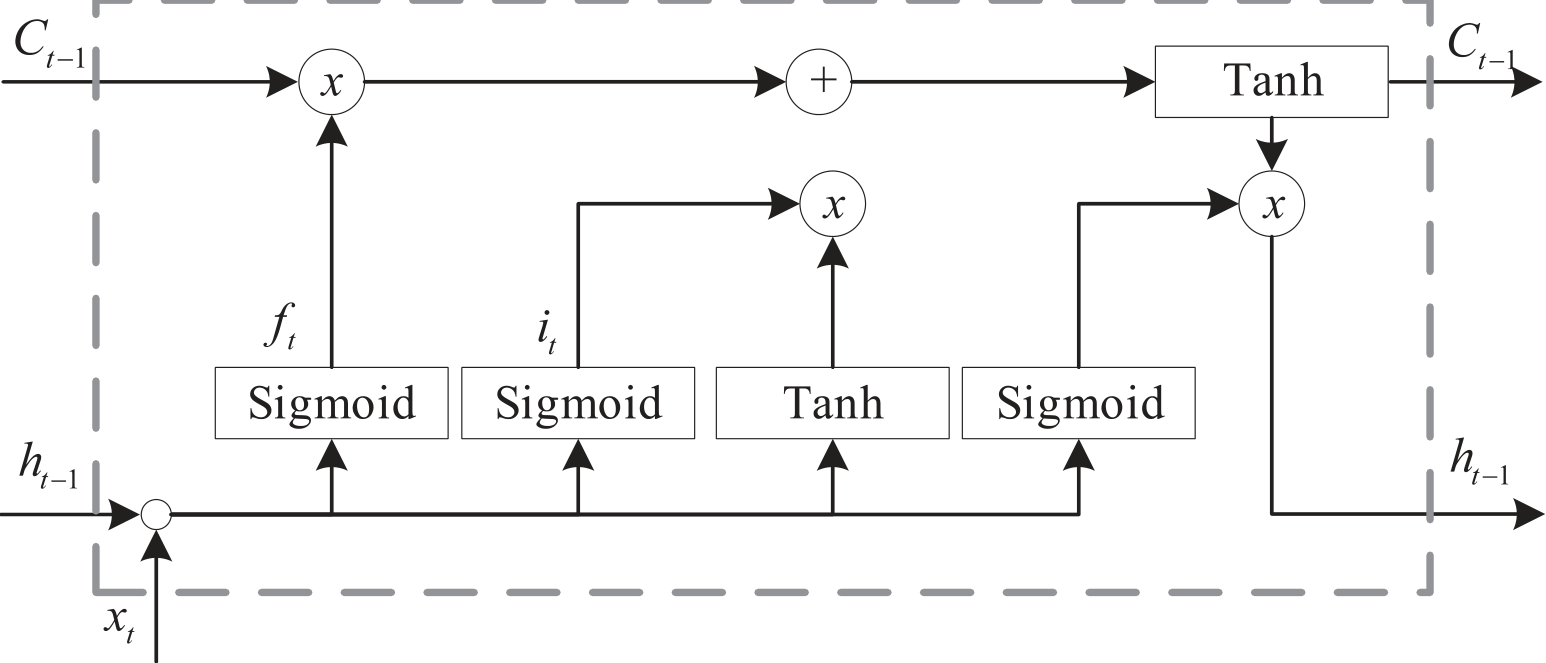
The LSTM algorithm can effectively address the gradient vanishing and explosion issues that standard RNNs are prone to when dealing with long-term dependency problems. Compared to standard RNN networks, the most important feature of LSTM networks is that they replace repetitive simple structural modules with memory cell units in hidden network structures, such as a tanh layer. This special interaction mode enables LSTM to learn long-term characteristics, thus realizing the function of long-term memory. LSTM is essentially still a neural network model, mainly composed of input, loop hiding, and output layers. The fundamental unit of the LSTM hidden layer is a special cellular structure, with each LSTM cell composed of three parts: input, output, and forgetting gates, which are used to protect and control information. As shown in Fig. 1, this is a single-layer hidden layer LSTM network cellular structure.
The function of the forgetting gate in LSTM is to screen the neuronal state information at k–1 time to determine whether it has an impact on the neuronal state at k time. The screening method is shown in Equation (1). According to the input xk at k moment, the state hk–1 at k–1 moment, and the Sigmaid activation function processing, it can get the output f(k) whose value is in the interval [0, 1]. The closer f(k) is to 1, the more high-value information the neuron state has, and it should be reserved to the next moment. On the contrary, the closer f(k) is to 0, the less high-value information it contains, and it should choose to forget or delete this information.
In Equation (1), σ, Wf, and bf are the parameters that need to be trained in LSTM. The input gate is mainly responsible for updating the neuron state at k time, and the detailed calculation is expressed in Equations (2) and (3). According to the input xk at k time and the state hk–1 at k–1 time, the input gate is activated by the tanh function to obtain Ck, and then calculated by the same Sigmoid activation function to obtain ik with a value in the interval [0, 1]. The size of ik determines the degree to which input information xk affects the state of neurons.
In Equation (2), Wc and bc are the LSTM parameters that need to be trained. The calculation method of ik is shown in Equation (3).
In Equation (3), Wi and bi are also the LSTM parameters that need to be trained. The output gate’s function is to control the output of the memory cell state, and it includes two parts. The first part of the output gate is worked out by the activation function Sigmaid through the input xk at k time and the state hk–1 at k–1 time; the second part of the output gate is calculated from the memory cell state Ck through the tanh activation function.
However, in predicting the concentration of air pollutants represented by PM2.5, the importance of input time series information varies. However, traditional LSTM algorithms silently process all input information in an average equal weight manner, which may affect the highlighting of high-value information in the model and lead to the model falling into local optima. So this study introduces AM into traditional LSTM and constructs an improved LSTM model. In the AM calculation process, the correlation of all LSTM neurons is scored according to the scoring function. The scoring function St calculation method is shown in Equation (4)
In Equation (4), LSTM( ) means the scoring function of the LSTM network, which is calculated based on cosine similarity. The Ct–1 calculation method is shown in Equation (5).
In Equation (5), αti means the total number of neurons in the current neural network when processing natural language tasks, and T indicates the probability of the importance of neuron hi. The calculation method is shown in Equation (6).
In Equation (6), N expresses the maximum number of the current input sequence, and eji is an intermediate variable. The calculation method is shown in Equation (7):
The meaning of f(st, hi) in Equation (7) is the hi mapping function with si in the neural network. The AM will automatically focus on important features and filter out useless features based on the weighted values of all LSTM neuron states and attention, thereby improving the efficiency of algorithm data processing.
This study selects the LSTM network as the basic prediction model and constructs an LSTM network structure consisting of an input, LSTM, sense, dropout, and output layers. The input of the LSTM network is a sequence data segment with a sliding time window of T, namely Xk = [x1, x2, x3, ..., xT]k. xT means the data of the Tth unit time, and Xk expresses the air pollution and meteorological data for consecutive T days. At each time point, the LSTM network not only receives input data x from the current time point, but also receives storage unit state ct–1 and hidden layer state data ht–1 from the previous time point, and dynamically recurs in the time dimension to form the final output data. The function of the dropout layer is to randomly remove hidden layer neurons with probability p to prevent overfitting caused by the joint action of feature detectors. However, considering the strong nonlinear and non-stationary characteristics of air pollution data such as PM2.5, a single LSTM network structure can only mine data signals from different time periods and the same dimension and cannot handle problems such as noise. Therefore, the CEEMD algorithm is now introduced for smoothing PM2.5 data, and a prediction model integrating CEEMD and the improved LSTM algorithm (LSTM-CEEMD) is designed. By introducing a pair of positive and negative paired, independent, and identically distributed random variables as auxiliary white noise into the CEEMD algorithm for noise collaborative analysis, the model effectively solves the problem of mode aliasing that is common in empirical mode decomposition (EMD) signal decomposition and eliminates redundant noise when the signal is reconstructed. The structure of the ILSTM_CEEMD model is denoted in Fig. 2. The steps of the ILSTM_CEEMD prediction model are as below: Firstly, it needs to standardize the input data. Secondly, the CEEMD algorithm is used to decompose PM2.5 raw data into multiple relatively stable components and trend items where it constructs an LSTM prediction model. The next step is to use the LSTM model to train and predict each component and trend item separately and continuously adjust the network parameters during the training and learning process. Input the prediction results of each component into the AM, which returns information to the LSTM network and outputs the final prediction outcomes of the model. During the establishment of the model, air pollutants such as PM10 and SO2 from the past T hours and meteorological data are selected as input variables to predict IMF components or trends for the next hour.
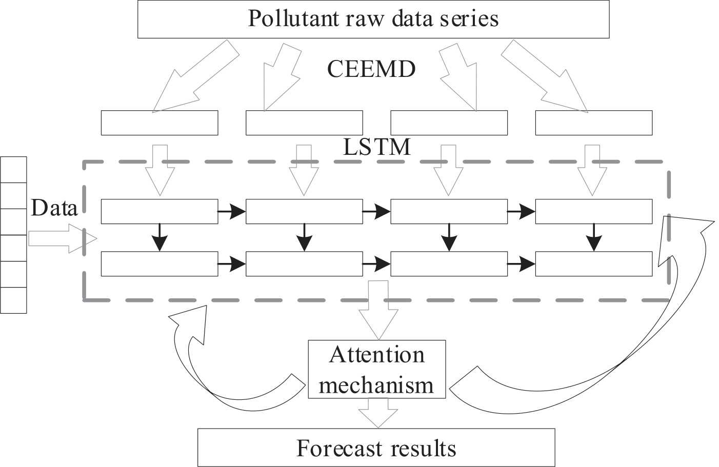
The AM is added to the prediction model between the LSTM algorithm’s computational structure and output steps. After completing this improvement, the AM will score the time series feature vectors processed by LSTM, select the feature vector with the highest score to retain, and calculate the context feature vector by the weighted average of all output feature vectors. Based on this, the candidate time series feature vectors will be assigned values, and the key sequences in the data will be identified to adjust the data processing focus of LSTM.
Improved UAPCP Model Integrating Spatiotemporal Optimization and Data Dimensionality Reduction
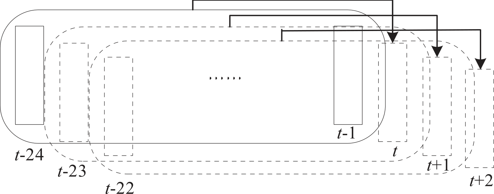
Since air pollutant concentration data is an indicator closely related to time and space, from the perspective of input data, the ILSTM_CEEMD prediction model is optimized based on time, space, and spatiotemporal factors to construct an ILSTM_CEEMD prediction model based on spatiotemporal optimization. To adapt to the input format of the LSTM model, the input data is adjusted to the matrix format of [samples, timesteps, features], where samples, timesteps, and features represent the samples, time steps, and total number of features for a training session. The size of T determines the impact of T hour historical pollutant data and meteorological data on model prediction. The calculation and movement of the sliding time window are expressed in Fig. 3.
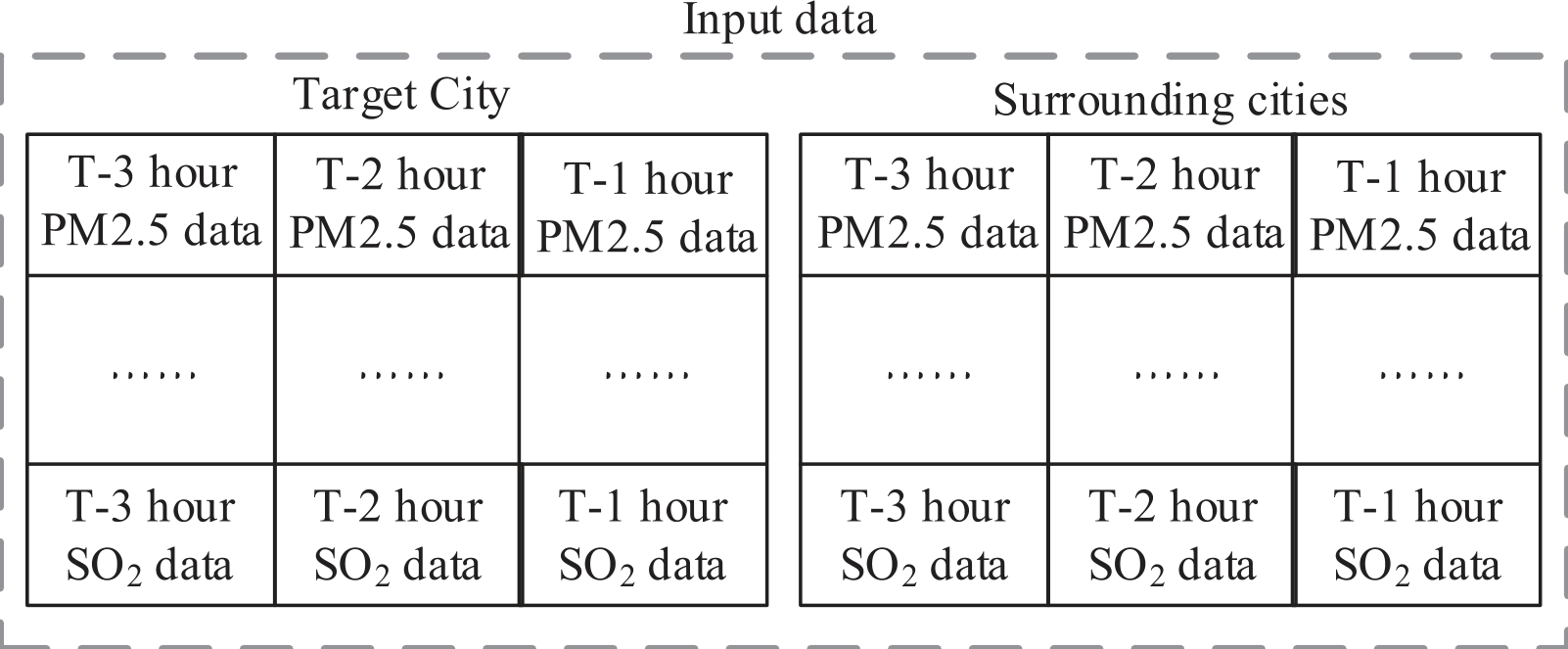
After multiple tests, the sliding time windows of 1, 3, 8, 12, and 24 have now been set to T. The above model only considers temporal characteristics and does not consider the impact of spatial factors on pollutant diffusion. For example, when serious high pollution incidents occur in surrounding cities, after a period of air transmission, the air quality of the target city will also be affected, and the concentration of air pollutants will increase accordingly. So the model is further optimized based on space; that is, the air pollution data of surrounding cities in the city where the dataset is located is also input into the model in the hope of improving the forecast accuracy and universality of the model in the region. The current ILSTM_CEEMD prediction model based on spatiotemporal optimization has only changed the data input part compared to the model in Fig. 2, as shown in Fig. 4. Where this is the input sample of the prediction model based on spatiotemporal optimization. Under this spatiotemporal optimization strategy, when predicting the concentration of PM2.5 air pollutants in a certain hour of the target city in the dataset, the input data of the model include air pollutants and meteorological data in the past T hours of the province and surrounding cities.
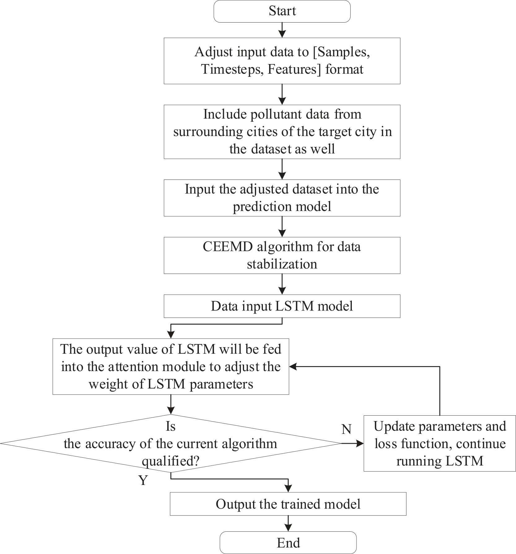
After introducing temporal and spatial information, the calculation process of the prediction model is shown in Fig. 5. As shown in Fig. 5, for the current prediction model, the input data needs to be processed three times, namely adjusting the data form for expanding the time dimension, adding data from surrounding cities, and using the CEEMD algorithm for stabilization.
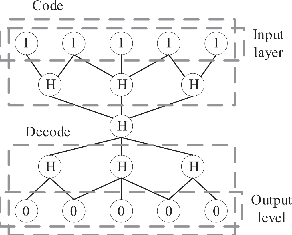
After introducing temporal and spatial information, the feature dimension of network input data significantly increases. Although further optimization can be achieved through feature extraction, the traditional dimension reduction algorithm can only linearly map the input data from high to low dimensional space, and cannot perform nonlinear mapping changes. Therefore, to enhance the feature learning ability of neural networks on feature data and improve the prediction performance of LSTM, SAE neural networks are now introduced. By utilizing the SAE neural network to compress and encode multidimensional feature data, a new prediction model is constructed. Auto Encoder (AE) can carry out feature learning on input information and is widely used in feature extraction and outlier detection. The main components of AE are the encoder and decoder. The encoding part is responsible for learning the input data’s implicit features. By minimizing the reconstruction error, the coding and decoding parts are continuously optimized to learn the abstract features of the original data and achieve the target of feature extraction. The computational structure of AE is shown in Fig. 6. The object marked “H” in Fig. 6 represents hidden layer neurons.
The AE structure sets the input and output layers to the same number of neurons. With the center as the boundary, the number of coding process neurons on the left is reduced layer by layer for data compression, while the decoding process on the right is used to increase the number of neurons layer by layer. By constantly modifying the parameters of the encoder and decoder, the reconstruction error is minimized, resulting in the reconstruction of input data and improving the recovery ability of original data. After the training is completed, the encoding result at the bottleneck is the extracted low dimensional feature values. The SAE neural network is a deep neural network constructed from multiple AE layers. Assuming the number of SAE layers is n, use W(k,1), W(k,2), b(k,1) and b(k,2) to stand for the parameters of the k th AE respectively. In each layer of AE, encoding operations are performed according to the execution sequence from front to back. This process can be described by the following Equations (8) and (9). Equation (8) is the calculation method for the activation value a(k) of the hidden layer unit in the k th layer.
In Equation (8), f(∙) is the encoding mapping function; z(k) indicates the upper layer neuron’ output; k denotes the current number of calculation layers. After calculating a(k), the output of this layer can be calculated according to Equation (9).
The SAE is also executed from back to front. In the SAE decoding process, it decodes the AE in the network layer by layer from back to front. The specific equation is described as follows, and Equation (10) is used to calculate the activation value a(n+k) of the hidden layer unit in the n+k th layer.
Fig. 5.
Prediction model calculation process after adding spatiotemporal characteristics to input data.
In Equation (10), g(∙) indicates the decoding mapping function. The next step is to calculate the output z(n+k+1) of the current decoding layer according to Equation (11).
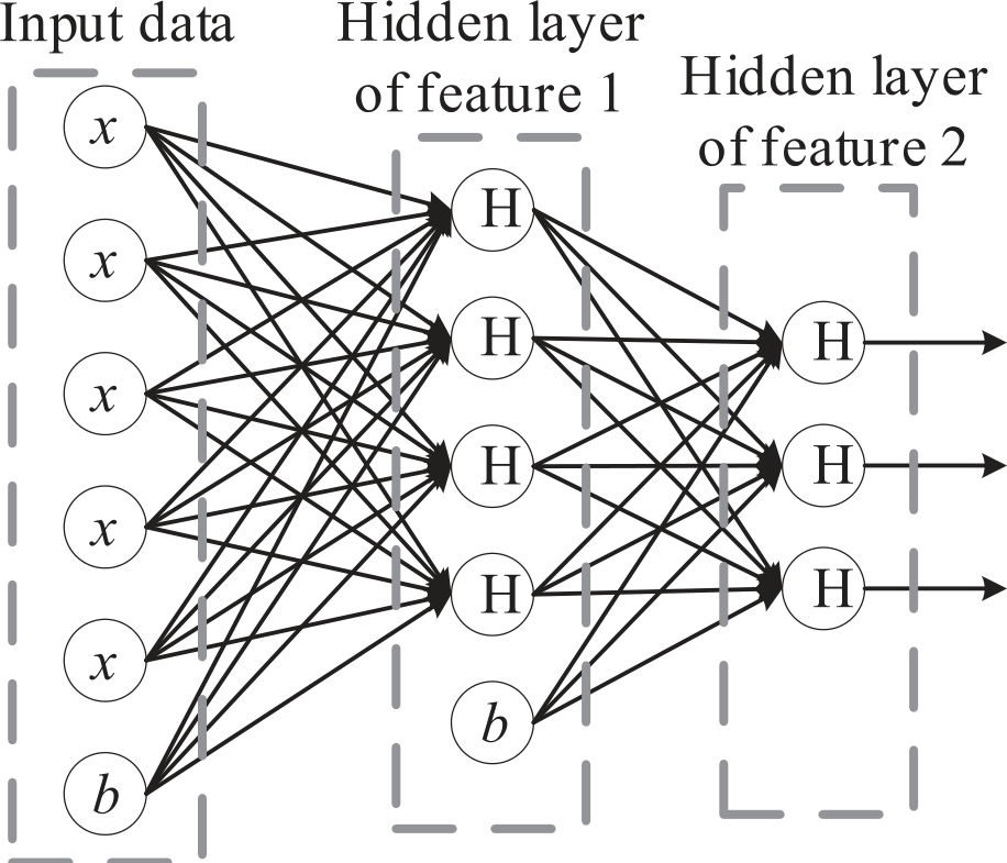
It calculates according to equations (10) and (11) to obtain a(n+k), which denotes the activation value of the deepest hidden unit. This output vector includes the key data that needs to be extracted. When dealing with classification problems, this output vector can serve as the input feature of the classifier. From this, the calculation structure of SAE can be obtained, as shown in Fig. 7.
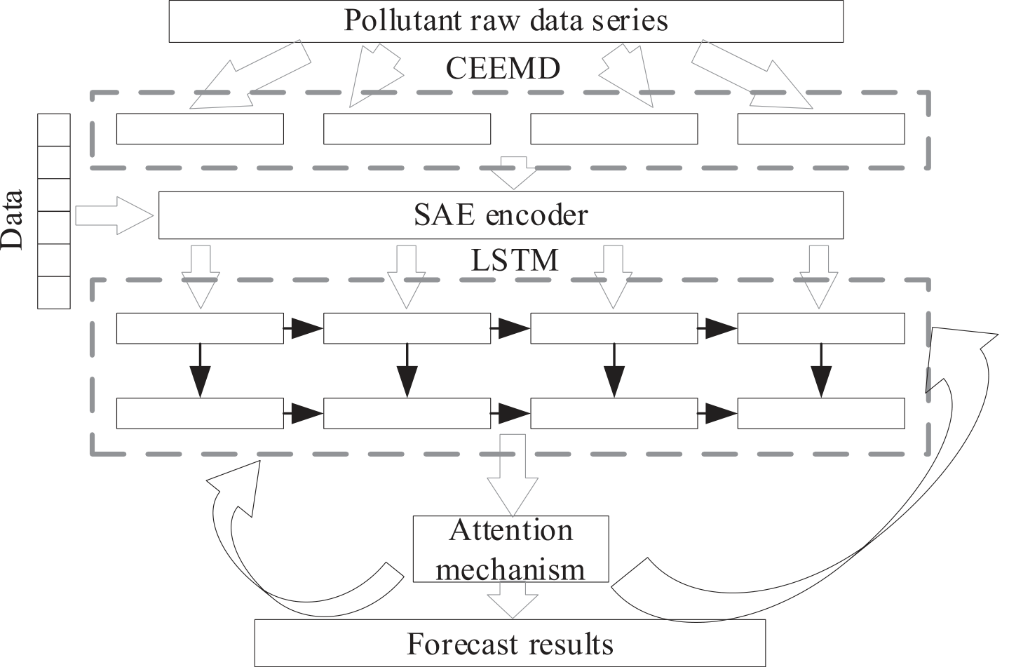
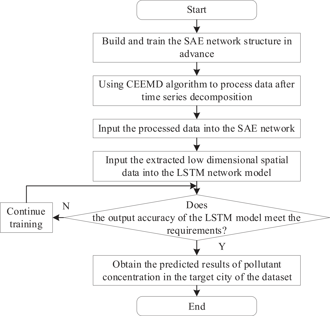
At this point, an improved prediction model for pollutant concentration can be obtained by introducing the SAE network. The model’s structure is shown in Fig. 8. Where this optimization model requires the pre-construction and training of the SAE network structure. Then, the CEEMD algorithm is used to process the decomposed time series data, as well as other raw air pollution and meteorological data, and the processing results are used as inputs to the SAE network structure. At the same time, the model also needs to limit the number of hidden layer neurons to be smaller than the input layer and use layer-by-layer greedy training method to train and learn multi-layer AE layer by layer. In the research, the SAE coding part is used for feature learning, and the air pollution data is compressed and encoded. The original high-dimensional feature data is equivalently mapped to the low dimensional space to realize the nonlinear mapping operation of feature data. Then, the extracted low dimensional spatial data is used as input for the LSTM network model, and the compressed and encoded data is used to explore potential patterns of information mining, ultimately obtaining the prediction results of pollutant concentrations in the target city of the dataset.
The calculation process of the urban air pollutant concentration prediction model designed in this study is shown in Fig. 9. As shown in Fig. 9, the first step of model calculation is to construct and train the SAE network. The second step is to preprocess the decomposed data using the CEEMD algorithm and then input the data into the SAE network. The third step is to input the low bit spatial data output from the previous step into LSTM. The fourth step is to determine whether the prediction accuracy of the current LSTM model meets the set requirements or whether the number of iterations has reached the maximum set value. If the judgment result is "yes", use the trained model to predict the test set data; otherwise, continue to iterate the LSTM model.
Finally, it designs the evaluation indicators needed in the model performance verification experiment. Considering that the model established in this study is essentially dealing with regression analysis, it chooses root-mean-square error (RMSE), mean absolute percentage error (MAPE), MAE, and R-Square (R2). The calculation method for RMSE is indicated in Equation (12).
In Equation (12), yi and ŷi denote the actual and predicted values of the sample data, and n refers to the total number of samples in the test data.
The calculation method for MAPE is expressed in Equation (13).
The calculation method for MAE is shown in Equation (14)
The calculation method of R2 is illustrated in Equation (15)
In Equation (15), ȳi expresses the average value of the sample data, while n represents the number of samples in the test data.
Results and Discussion
To test the forecast accuracy of the mixture model on the concentration of air pollutants, an experiment was now designed and carried out. The experimental data set came from the air quality data of Changsha-Zhuzhou-Xiangtan. These data were the average concentrations of pollutants per hour, and the measurement time stamp was 24 hours a day. To adapt to the input format of the neural network and promote the accuracy of the prediction model, the following pre-processing methods were needed for the original data: the pre-processing methods used were to fill in missing values according to the linear interpolation method, to normalize the data, and to segment the time series according to the sliding window method with a step size of 1.
Experimental Plan Design
After processing the dataset results, a total of 115367 pieces of data were included, and the experimental and test sets were divided in a 7:3 ratio, resulting in a test containing 34610 pieces of data. The experiment was mainly divided into two parts. The first part was mainly to evidence the performance of the improved parts of the model, and the second part was to prove the performance level of the designed model with the best practical effect compared to other models. In the first part of the experiment, the selected solutions included the traditional LSTM algorithm, the improved LSTM (ILSTM) algorithm that integrated AM, the spatiotemporal optimization+ILSTM (S_ILSTM), and the model constructed by the improved LSTM algorithm that also includes spatiotemporal optimization and SAE (SAE_S_ILSTM). In the second part of the experiment, the selected comparison models were constructed according to the gated current neural network (GRU) and RNN algorithms commonly used in time series information processing, and the parameters of various RNNs were determined according to the method of multiple debugging to obtain the optimal results. The parameter schemes used in the final research and design model are shown in Table 1.
Analysis of Experimental Results
Firstly, it compared the ILSTM algorithms with the prediction models constructed by the LSTM algorithm itself. The changes in MAE and R2 indicators during the training phase are displayed in Fig. 10. The horizontal axis in Fig. 10 represented the number of training sessions, while the vertical axes in subgraphs (a) and (b) denoted MAE and R2, respectively. Line styles were used to distinguish different algorithm models. Observing Fig. 10, as the number of iterations increased, the changes in MAE and R2 indicators of each LSTM algorithm were completely opposite. MAE quickly decreased by several orders of magnitude before completing convergence, and R2 indicators also tended to converge after rapid growth. The MAE and R2 indicators of LSTM, ILSTM, S_ILSTM, and SAE_S_ ILSTM algorithms after training were 9.1, 8.3, 4.5, 4.0, and 0.82, 0.88, 0.93, and 0.94, respectively.
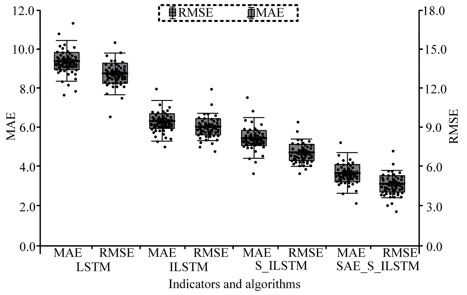
Compare the MAE and RMSE values of these trained LSTM algorithms on PM2.5 pollutants and reduce the difficulty of display, only 50 sample points were randomly selected for plotting. In Fig. 11, the horizontal axis represents the algorithm and evaluation indicators, and the black dots represent the data points. Observing Fig. 11, the LSTM algorithm had the highest overall MAE and RMSE values on the selected test set samples, while the prediction accuracy was the worst. The accuracy of the ILSTM and S_ILSTM algorithms was higher than that of the original algorithm, while the overall accuracy of the SAE_S_ILSTM algorithm was the highest. The median MAE and RMSE of LSTM, ILSTM, S_ILSTM, and SAE_S_ILSTM algorithms on selected samples were 8.8, 5.7, 4.9, 3.7, and 14.1, 9.5, 7.8, and 5.6, respectively.
The performance of each LSTM algorithm on the overall test set is indicated in Table 2. From Table 2, the unmodified LSTM performed the worst on various accuracy indicators. The SAE_S_ILSTM algorithm, which included all improvement measures, performed significantly better on various accuracy indicators than other LSTM algorithm models. However, in terms of computational time, the algorithm that adjusted the data format according to the algorithm and data characteristics and incorporated AM had the shortest computational time, while the SAE_S_ILSTM algorithm had slightly lower computational efficiency due to the addition of the SAE network.
Table 1.
SAE_S_LSTM model parameter scheme.
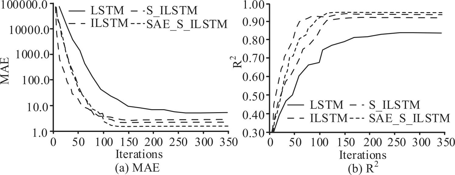
Table 2.
Performance of each LSTM algorithm on the overall test set.
| Index | LSTM | ILSTM | S_ILSTM | SAE_S_ILSTM |
|---|---|---|---|---|
| MAE | 9.8 | 7.2 | 7.1 | 6.7 |
| RMSE | 14.8 | 12.3 | 9.9 | 9.2 |
| MAPE | 25.4 | 14.9 | 15.2 | 8.6 |
| R2 | 0.88 | 0.90 | 0.91 | 0.93 |
| Calculation time (s) | 12.75 | 4.92 | 4.25 | 6.07 |
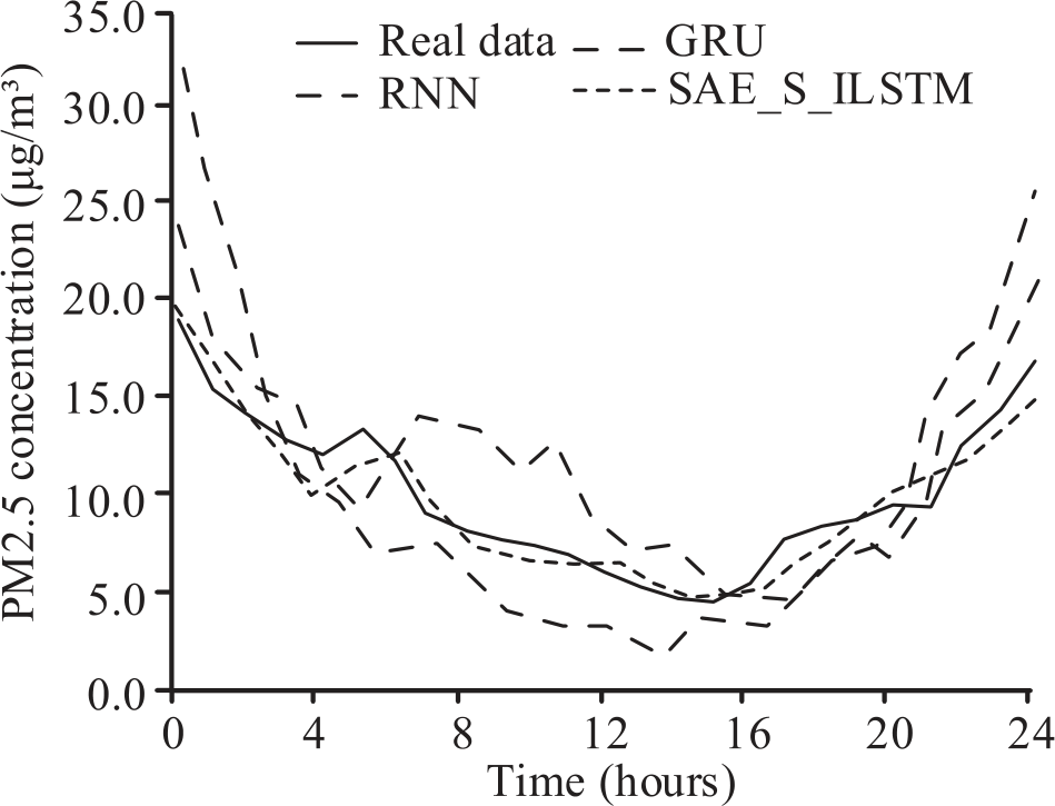
In summary, the SAE_S_ILSTM algorithm model had the best overall prediction quality, and this model was selected for comparative analysis with other different types of RNN algorithm models. It randomly selected 24-hour data from the dataset for intuitive prediction performance comparison, as expressed in Fig. 12. The horizontal axis of Fig. 12 is the measurement time of the data on that day, while the vertical axis expresses the concentration value of PM2.5. The solid black line represents the actual PM2.5 concentration, and the other three styles of lines represent different prediction models. Observing Fig. 12, the PM2.5 concentration was the lowest around 3pm on that day and the highest in the early morning. The predicted results of each model captured this pattern, but overall, the SAE_S_ILSTM algorithm designed in this study predicted results that were closest to the real data.
Next, it will attempt to compare the performance of each prediction model from a quantitative analysis perspective. Firstly, it compared the forecast accuracy of the model under different prediction sample sizes to determine the stability of each model. The statistical outcomes are displayed in Fig. 13. Observing Fig. 13, as the number of samples participating in the calculation increased, the fluctuation of calculation errors for each algorithm gradually decreased, but the overall fluctuation amplitude of the SAE_S_ILSTM algorithm was the smallest. Specifically, the MAE and RMSE of SAE_S_ILSTM, GRU, and RNN algorithms on the entire test set were 6.7, 9.3, 10.8, and 9.2, 13.6, and 17.2, respectively.
A comparison of the memory consumption data of each model is shown in Fig. 14. Observing Fig. 14, as the number of samples to be calculated increased, the memory consumption of each model showed a trend of rapid growth followed by a slowdown in growth rate. Although the SAE_S_ILSTM algorithm designed in this study had a total computational time of 48 MB when calculating the sample size, which was higher than the other two models, the memory consumption growth rate of this model was the lowest. When the sample to be calculated was the entire test set, the computational memory consumption of the SAE_S_ILSTM, GRU, and RNN algorithms was 81 MB, 117 MB, and 154 MB, respectively.
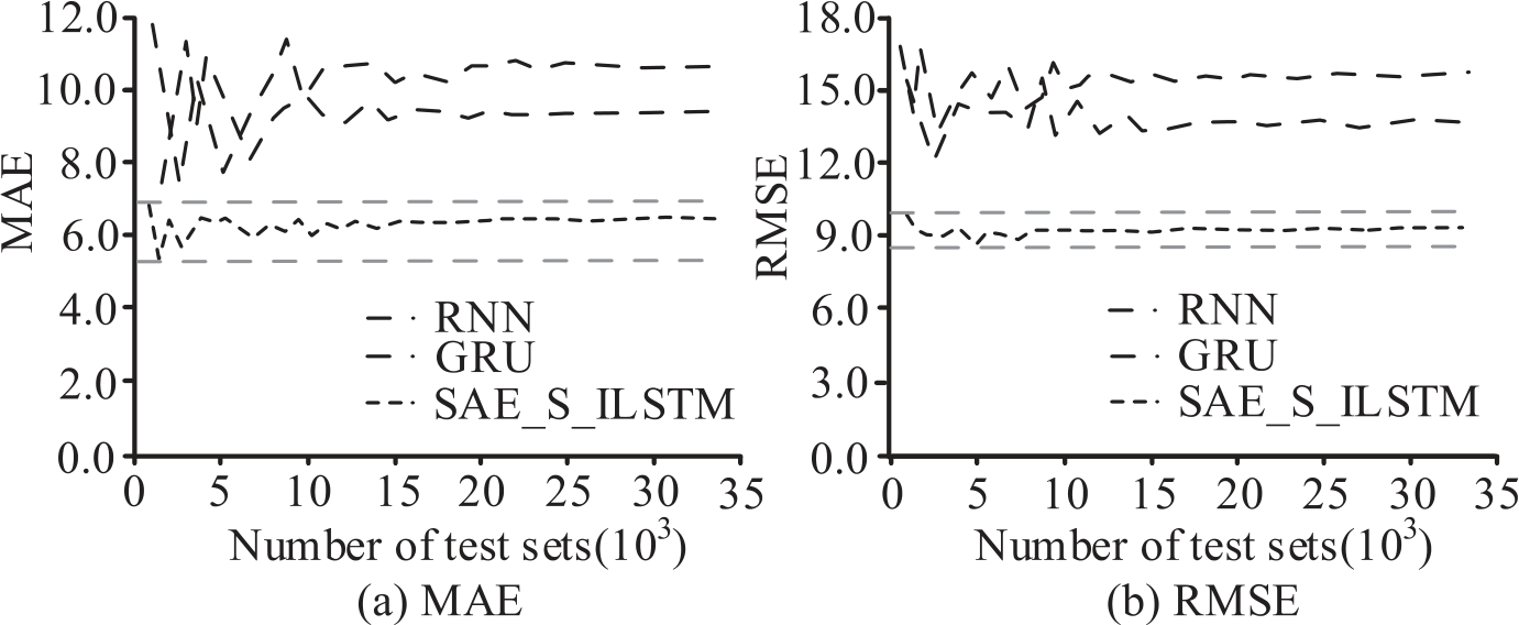
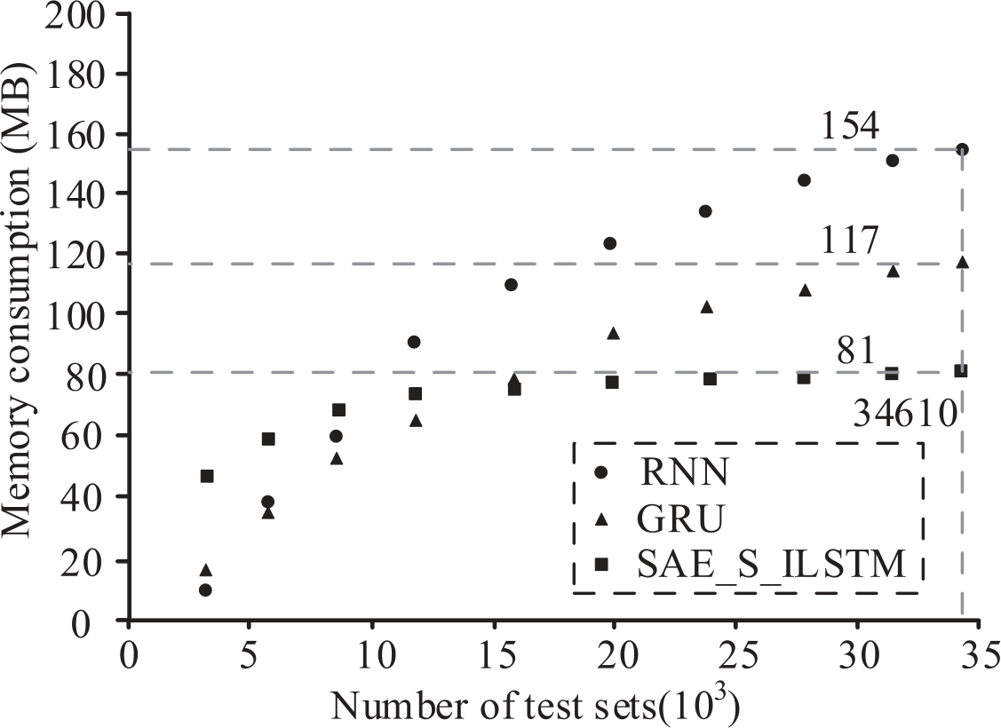
Table 3.
Comparison of various indicators of each model on the overall test set.
| Indicator number | Index | RNN | GRU | SAE_S_ILSTM |
|---|---|---|---|---|
| #1 | MAE | 10.8 | 9.3 | 6.7 |
| #2 | RMSE | 17.2 | 13.6 | 9.2 |
| #3 | MAPE | 28.2 | 17.5 | 8.6 |
| #4 | R2 | 0.82 | 0.91 | 0.93 |
| #5 | Calculation time (s) | 3.18 | 4.81 | 6.07 |
| #6 | Memory consumption (MB) | 154 | 117 | 81 |
Table 4.
Comparison of Prediction Ability of Excellent Methods in Multiple References.
| Index | Method of Reference | Method of Reference [18] | Method of Reference [19] | SAE_S_ILSTM |
|---|---|---|---|---|
| MAE | 26.8 | 8.5 | 10.3 | 6.7 |
| RMSE | 52.6 | 15.3 | 22.9 | 9.2 |
| MAPE | 74.6 | 18.7 | 25.2 | 8.6 |
| R2 | 0.74 | 0.84 | 0.81 | 0.93 |
| Calculation time (s) | 3.15 | 12.7 | 8.25 | 6.07 |
Finally, by comparing the changes in various evaluation indicators of each model on the overall test set, as shown in Table 3. Observing Table 3, the performance of SAE_S_ILSTM designed in this study on MAE, RMSE, MAPE, and R2 indicators was superior to the other two prediction models, with less memory consumption than the other two models, but the calculation speed was slower than the other two models.
In order to enhance the scientific nature of the research, the horizontal prediction ability of the designed model is now being compared with excellent prediction models from multiple references. The statistical results are shown in Table 4. The data in Table 4 were calculated using their respective literature test sets. Observing Table 4, it can be seen that the prediction model designed in this study is superior to the other three methods in terms of accuracy indicators, and the calculation time is only second to that of reference [17]. This is because the method designed in reference [17] is based on an improved traditional time series calculation model, which has fewer computational processes and lower computational complexity. However, the disadvantage is that it has very poor processing ability for data with nonlinear relationships. The method designed in reference [18] showed relatively good predictive performance because it took into account information such as the historical concentration and particle size range of the predicted gas during the design process, effectively reducing the possibility of information misjudgment. The prediction accuracy of reference [19] is also relatively good, as it uses kernel fuzzy mean to cluster the data, and designs backpropagation neural network concentration prediction models using genetic algorithm optimization parameters according to the clustering results, so that the prediction model can globally optimize and solve different categories of gases. However, the models in references [17], [18], and [19] also failed to consider the spatiotemporal characteristics of gases.
In summary, considering that the forecast accuracy of this model is superior to traditional models, it can be used to predict the concentration of urban air pollutants and, combined with expert evaluation experience, provide residents with more accurate and practical air quality and key pollutant warnings for travel, outdoor tourism, and office matters.
From the experimental results of this study, it can be seen that, compared to the traditional LSTM algorithm, the improved algorithms show significant improvements in key performance indicators such as MAE and R2. The SAE_S_ILSTM model outperforms other models in all evaluation indicators, demonstrating its efficiency and accuracy in dealing with urban air pollutant prediction problems.
The SAE_S_ILSTM algorithm effectively captures complex patterns in air pollution data using SAE and improved LSTM networks. The advantage of this structure is that it can provide more accurate predictions while maintaining lower memory consumption. However, the drawback of this model is its relatively slow computational speed, which may be due to the addition of SAE increasing the complexity of the model.
The paper also mentioned experiments comparing the performance of the model under different conditions. For example, comparing the prediction accuracy of models under different sample sizes, the results indicate that the SAE_S_ILSTM algorithm has the smallest error fluctuation, which means it has the best stability when dealing with datasets of different sizes.
In addition, compared to other types of RNN algorithms such as GRU and RNN, SAE_S_ILSTM performs well on multiple evaluation metrics, especially when dealing with time series data such as PM2.5 concentration prediction. This has been confirmed in the comparison of intuitive prediction effects.
Finally, despite the fact that the SAE_S_ILSTM algorithm has performed well in current research, it has not been widely tested in cities with different latitudes and geographical environments. Future research can explore the impact of these factors on model performance, further optimizing and adjusting the model to adapt to different environmental conditions.
Overall, the significant contribution of this study lies in providing a high-precision urban air pollutant concentration prediction model, which is of great significance for urban planning, public health, and environmental protection. At the same time, it also provides valuable insights for subsequent research, especially in the use of deep learning techniques to process environmental monitoring data.
In addition, this study also demonstrated added value in the following aspects: Firstly, at the application level, this study also provides an effective tool for the field of urban planning. Decisionmakers in urban planning can use the output results of this model to understand the spatiotemporal distribution of air pollutants in the city, so that in future urban construction, densely populated areas can be moved away from high pollution areas, and green air purification belts and equipment can be installed in high pollution areas. This helps to improve the health and quality of life of residents. From the perspective of academic value, this study demonstrates the potential of deep learning in processing complex environmental data by combining LSTM and SAE, enriching the theoretical and practical applications of deep learning models in the field of environmental science. This study provides new ideas for future research in algorithm design.
Conclusions
The construction of HUS cannot be separated from air quality prediction services. To improve the accuracy of UAPCP, this study has designed an intelligent prediction model based on an ILSTM algorithm. The performance of the model was tested using real urban air pollutant data. The test outcomes indicated that the MAE and R2 indicators of LSTM, ILSTM, S_ILSTM, and SAE_S_ILSTM algorithms after training were 9.1, 8.3, 4.5, 4.0 and 0.82, 0.88, 0.93, and 0.94, respectively. The median MAE and RMSE of LSTM, ILSTM, S_ILSTM, and SAE_S_ILSTM algorithms on selected samples were 8.8, 5.7, 4.9, 3.7, and 14.1, 9.5, 7.8, and 5.6, respectively. The comparison findings of various LSTM algorithms on the overall test set denoted that the SAE_S_ILSTM algorithm, which included all improvement measures, performed significantly better than other LSTM algorithm models in various accuracy indicators. It selected the SAE_S_ILSTM algorithm model to compare and analyze with other different types of RNN algorithm models, and the results were as follows: As the number of samples participating in the calculation increased, the fluctuation of calculation errors for each algorithm gradually decreased, but the overall fluctuation amplitude of the SAE_S_ ILSTM algorithm was the smallest. Specifically, the MAE and RMSE of SAE_S_ILSTM, GRU, and RNN algorithms on the entire test set were 6.7, 9.3, 10.8, and 9.2, 13.6, and 17.2, respectively. At this time, the memory consumption was 81 MB, 117 MB, and 154 MB, respectively. The overall comparison findings indicated that SAE_S_ILSTM performed better than the other two prediction models in MAE, RMSE, MAPE, and R2 indicators and had lower memory consumption than the other two models, but its calculation speed was slower than the other two models. From the perspective of research value, the model designed in this study can output more accurate predictive data, providing a high-quality reference for expert analysis and thus providing better air health risk assessment services for residents. From the perspective of practical application value, the designed model can be used to design high-precision urban pollutant concentration prediction equipment. However, the drawback of this study is that it failed to test the application effect of the model in various cities with different latitudes and geographical environments, which is also a key focus for future research.