

Introduction
In today’s society, the process of urbanization is constantly accelerating, injecting new vitality into modernization construction, and socio-economic development. Meanwhile, it also brings a series of environmental problems, one of which is the issue of urban rainwater discharge. With the intensification and verticalization of cities, the design and operation of rainwater drainage systems are becoming increasingly prominent. Especially during rainy and heavy rain seasons, drainage systems often become blocked, leading to urban waterlogging and having a serious impact on urban operations and residents’ lives [1- 3]. Therefore, how to effectively solve the problem of rainwater discharge in the context of large-scale urbanization construction has become an important issue in current urbanization construction. Previous research has mainly focused on traditional surface and sewer drainage systems, often only able to cope with normal rainfall conditions. During heavy rain seasons, the drainage system often operates poorly, and frequent maintenance and repairs also bring significant economic pressure [4-6]. Recently, researchers have begun to pay attention to single bucket rainwater siphon drainage systems (SDS). This system, with its unique drainage mechanism and superior performance, provides new possibilities for solving urban rainwater drainage problems. The single bucket rainwater SDS is a new type of drainage technology that has advantages such as strong treatment capacity, fast response, and good drainage effect. More importantly, the system can adaptively adjust drainage on the ground during rainfall, thereby effectively reducing the occurrence of urban waterlogging. In addition, the system also has the advantages of easy installation, energy conservation, environmental protection, and low maintenance costs [7-9]. However, despite the many advantages of a single bucket rainwater SDS, there are still many areas for further research in terms of performance analysis and optimization design. Carrying out rainwater management to improve environmental protection, among which a single bucket rainwater siphon drainage system is an effective management method that can effectively reduce urban drainage load. The principle of this drainage system is to use pressure differences to achieve the treatment and discharge of surface water. The siphon drainage system, as a diversion type drainage system, can directly discharge rainwater from the source to the designated area, and it varies due to environmental and usage conditions. Therefore, further optimization is needed to better meet the urban scale of large spaces and improve drainage efficiency and reliability. There is still a lack of research and analysis on the development trend of flow rate in siphon drainage systems. The accuracy of results such as siphon start time and drainage flow rate in traditional numerical simulations is poor, and there is a lack of more accurate theoretical calculation methods. In addition, there is a lack of relevant explanation on the impact of commonly used suspension pipes on siphon drainage systems in existing buildings. Therefore, with the aim of improving urban drainage efficiency, improving the performance of siphon drainage systems, and enriching the relevant theoretical content of this drainage system, this study proposes a performance analysis of a single bucket rainwater siphon drainage system in a large space urbanization construction environment, aiming to provide suggestions for urban construction. The first part of the study introduces the purpose of the research. The second part designs a simulation model and an experimental platform. The third part conducts simulation and comparative analysis. The fourth part draws research conclusions.
Related Works
Recently, research on SDSs has gradually deepened. The Tohari team conducted on-site experiments on the stability of volcanic geological landslide zones in West Java Province to evaluate the effectiveness of SDSs. After observing for a year, it was found that the SDS significantly reduced the groundwater level and effectively prevented the groundwater level from rising during the rainy season. This significantly improves the long-term stability of landslide areas. For this reason, they conducted an in-depth evaluation of the factors that affect the effectiveness of siphon drainage [10]. The Yu team proposed a new solution that utilizes the siphon drainage method to stabilize the slope of the reservoir bank and verified it with the Shuping landslide in China. When the reservoir water level drops, the SDS will automatically start, reducing the groundwater level and leakage force on the slope. After digital simulation verification, this system is superior to traditional horizontal drainage systems in preventing instability caused by excessive leakage force [11]. The Lv team has designed a three-dimensional digital siphon drainage simulation method that can simulate the dynamic process of siphon drainage and provide a more effective drainage layout comparison method. In the application validation of sand dune village landslides in China, it was shown that this method has a significant effect on the impact of parameter settings on drainage effectiveness [12]. The Chen team has proposed a new method to prevent foot leakage and erosion on loess slopes. This method prevents the leakage and erosion of groundwater at the foot of the loess slope by combining filter pipes and siphon drainage. The experimental results indicate that this method has a certain range of influence on loess, so the layout of the equipment can be optimized through on-site testing [13]. The Shuai team proposed a self-initiated drainage method as a solution to the long-term and efficient drainage capacity issues of traditional drainage methods. This new method can automatically initiate drainage, generate a vacuum tube, and transmit it to the surrounding soil to form a saturated zone. This can improve the stability of the slope [14].
The application of VOF models in various fields is gradually deepening. Liu et al. Studied the water management simulation of proton exchange membrane fuel cells. They added micro ribs to the surface of the gas diffusion layer to improve water management efficiency. The numerical simulation results show that at a certain height, width, and contact angle, micro ribs can eliminate liquid water from the GDL surface through the capillary effect. Meanwhile, it can also improve the oxygen diffusion efficiency and enhance the output performance of fuel cells [15]. Xu et al.’s research focused on two-dimensional multiferrous material VOF monolayer films. They found that VOF thin films have both good ferromagnetism and excellent ferroelectricity, mainly attributed to Jahn Teller distortion. Their research suggests that by applying 4% compressive strain, the Curie temperature of VOF monolayer films can be increased to room temperature. This combination of ferromagnetism and ferroelectricity provides a potential platform for studying multiferrous effects and producing the next generation of multifunctional nanoelectronic devices [16]. Zhang et al. used the Euler fluid volume (FV) fraction model to simulate the impact cavity and gas-liquid two-phase flow in the top and bottom gas-fired converters. They added bubble induced turbulence terms to the equation through user-defined functions. Their research has shown that the Euler fluid VOF model has better performance than the particle track model in predicting gas-liquid two-phase flow [17]. The Burdaron team studied the surface fluctuations of liquids with different viscosities driven by wind. They added initial noise disturbances to the model to study their impact on interface evolution. Their research revealed the effects of wind speed and liquid viscosity on interface disturbances, streamline patterns, and energy spectra [18].
Various research teams have conducted in-depth research on the advantages of SDSs in reducing groundwater levels and preventing groundwater levels from rising during the rainy season. These studies have achieved positive and significant results, undoubtedly pointing out new directions for research in this field. However, not all places have mountain slopes or soil environments. Large spaces such as buildings and roads in cities also require effective drainage systems to cope with the problem of water accumulation caused by rainfall, which has not received sufficient attention. Therefore, to fill the gap in the field of SDSs, this study will analyze the single bucket rainwater SDS in the context of large-scale urbanization construction.
The Calculation Model and Experimental Design of Single Bucket Rainwater SDS
The research focuses on the design and experimentation of an operational model for a single bucket rainwater SDS. Firstly, a simulation operation model was studied and designed, followed by the construction of a full-scale single SDS experimental platform. The key point analysis mainly focused on the influence of the length of the suspension pipe (SPL).
Design of a Simulation Operation Model
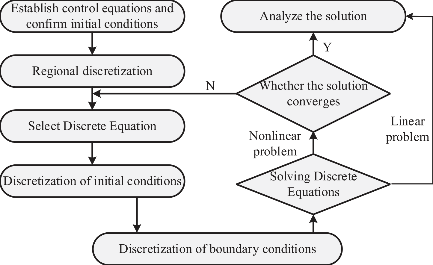
This study first analyzes the numerical calculation method of an SDS, which is solved by replacing the continuous domain of physical quantities with a set of discrete values. These discrete values represent discrete points in spatial and temporal coordinates. It uses specific principles to establish algebraic equations (discrete equations) for the values of these discrete points and variables and obtains approximate values of the required variables by solving these equations. The model operation process is shown in Fig. 1.
The essence of numerically solving physical problems is to replace the continuous field of physical quantities in time and space coordinates systems, such as the temperature field of a thermally conductive object, with a set of values on a finite number of discrete points. By solving an algebraic equation about common values established by a certain method, the value of the physical quantity being solved at the discrete point can be obtained. After spatial partitioning of the solution area, algebraic equations for physical quantities on nodes can be established based on actual needs. Determining whether the discrete equation is a linear problem plays an important role in the authenticity and reliability of the numerical solution results, and the solution situation may also be different [19]. The equation solving process for linear problems is more direct and simple, with lower computational complexity, stability, and uniqueness under specific conditions. When solving nonlinear problems, numerical methods are often used for approximate solutions, which may have multiple solutions, and the solving process is more complex. The convergence judgment of nonlinear discrete equations is related to the reliability and effectiveness of numerical solutions. Only when the iterative solution region converges can the obtained numerical results tend to be more realistic, and the algorithm can avoid getting stuck in meaningless iterative processes, achieving a better understanding of the problem. In terms of control equations, this study mainly uses mass conservation equations, momentum conservation equations, and energy conservation equations to describe flow and heat transfer problems. The conservation of mass equation is a continuity equation, as shown in formula (1).
In formula (1), ρ serves as the density of the fluid. t is
∂ time. is the partial derivative of time. u is the
∂t velocity vector of the fluid, and div is the divergence of density flow in the velocity field. Formula (1) can be simplified into the form of formula (2).
The formula for the conservation of kinetic energy can be divided into three directions. The formula for the x direction is shown in formula (3).
In formula (3), u' denotes the flow velocity component in the direction of x, SMx denotes the fluid source in the direction of x, and μ denotes the hydrodynamic viscosity. The formula for the y direction is shown in formula (4).
In formula (4), v denotes the flow velocity component in the y direction and SMy denotes the fluid source in the y direction. The formula for the z direction is shown in formula (5).
In formula (5), w denotes the flow velocity component in the z direction and SMz denotes the fluid source in the z direction. Formulas (3) ~ (5) satisfy the conditions of equation (6).
The energy conservation equation under this condition is shown in formula (7).
In formula (7), i denotes the fluid internal energy, k denotes the thermal conductivity, si denotes the heat source, Φ denotes the dissipation function, and p' denotes the fluid pressure.The equation of state for an ideal gas is shown in formula (8).
In formula (8), T represents temperature and R represents the gas constant. The turbulent kinetic energy equation is shown in formula (9).
In formula (9), σk is a constant, and the more applicable constant is 1.00. ε is the dissipation rate, u is the mean velocity, t is the time, and PG denotes the gravitational pressure of the fluid. The turbulent kinetic energy dissipation rate equation is shown in formula (10).
In formula (10), μt represents the hydrodynamic viscosity per unit time. σε is a constant with a high degree of applicability of 1.30. C1 denotes the empirical constant 1, which commonly takes the value of 1.44, and C2 is the empirical constant 1, which commonly takes the value of 1.92.
This study established a geometric size model that conforms to the actual situation in the computational fluid dynamics calculation software STAR-CCM+. In the boundary conditions of the calculation area, a pressure outlet is set, and the air volume fraction is 1. The simulation structure is shown in Fig. 2.
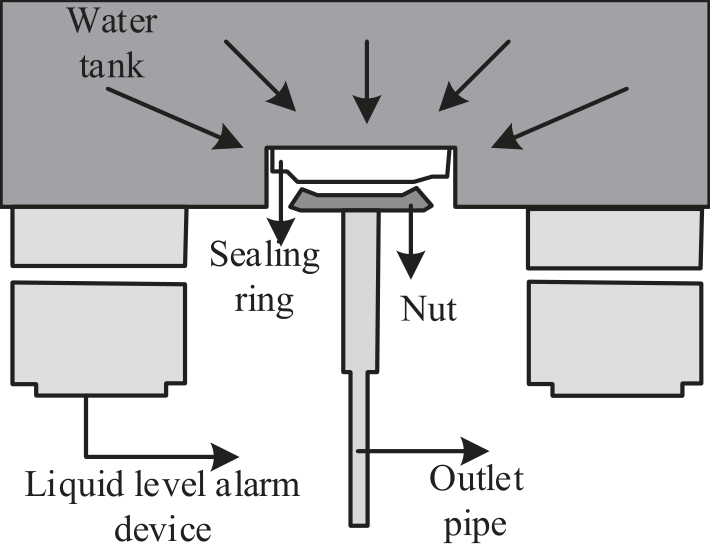
Fig. 2 is a schematic diagram of the initial liquid level structure of the water tank. The liquid level structure of the water tank includes five parts: the water tank, sealing ring, nut, liquid level alarm device, and outlet pipe. In addition, a constant flow input is set at the pipe openings at both ends of the top of the water tank (WT). It sets the water volume fraction to 1, while adding a water replenishment amount that matches the demand. To calculate the changes in FV and determine the FV function for the current unit at the next moment, as well as the way FV changes between adjacent units, staggered grid technology was used in the study. The study introduces a VOF model that links the changes in FV with the motion of particles. Assuming the existence of any function f(x, y) , there is formula (11).
(11)
The average value of f in the calculation unit is shown in formula (12).
In formula (12), (x, y, t) represents the spatiotemporal coordinates, and the integral form of the formula can be obtained as shown in formula (13).
The flow volume changes over time using a first-order forward difference scheme, as shown in formula (14).
In formula (14), both δFi+1, j and δFi,j +1
2̄ 2̄ represent volumetric flow rates. In the calculation process, special attention needs to be paid to the definition of the primary and secondary phases. In this study, continuous water flow is considered the main phase, while air dispersed in the main phase is considered the secondary phase. To accurately track and calculate various physical quantities during flow, it is necessary to set a reasonable time step. To continuously optimize the model and perform precise verification, sections and points were also set up at different locations to monitor pressure and flow. The selection of these positions is based on the working principles of the actual siphon system and possible changes.
Method of Setting Up Comparative Experiments
This study aims to establish a full-scale single SDS experimental platform and use indirect measurement methods to study the siphon drainage process. The purpose of the experiment is to study the variation in the state of flow inside this pipe under different water replenishment conditions, as well as the dynamic changes in pressure, drainage, and gutter water level inside the pipe. The experimental results will provide a basis for subsequent numerical calculation research. This experimental platform consists of two main parts: an SDS as well as a water replenishment system. The operation mode is shown in Fig. 3.
The SDS includes a top WT, a siphon rainwater bucket, and drainage pipes. The top WT is similar to the gutter in actual engineering. It has a water storage function and is equipped with a transparent PVC hard plastic plate, which facilitates the observation of internal rainwater flow patterns and liquid level changes. The commonly used TY56 type siphon rainwater bucket is selected, and the corresponding size is selected on the ground of the rated drainage capacity calibrated by the manufacturer [20-22]. The drainage pipeline adopts suspended pipes and is designed to be laid without slope. All drainage pipes are made of transparent U-PVC vfmaterial, making it easy to observe the water flow status vf dx inside the pipes (Table 1).
The replenishment system mainly includes a bottom WT, replenishment pipeline, water pump, and other equipment. The bottom WT adopts an open design for storing and providing make-up water. The water pump is responsible for lifting the water from the bottom tank to the top tank, and completing real-time water replenishment work [23-25]. The research aims to obtain dynamic changes in the siphon drainage process, including real-time flow state changes, pressure changes, and displacement changes in the drainage pipeline. High-speed cameras are used for flow monitoring, and color substances that do not affect water quality are added to the water to record the flow picture more clearly. It selects multiple recording points on the suspension pipe to observe changes. It installs a pressure transmitter at the suspension pipe to test the negative pressure change inside the pipe. Due to the need to test the static pressure of the pipeline, a static pressure tapping hole perpendicular to the pipeline is opened at the top of the pipeline during installation, and then the tapping hole is connected to the pressure transmitter through a plastic hose. Due to the presence of water air two-phase flow during the siphon drainage process, it is difficult to test real-time flow through a flow meter. Therefore, in this experiment, an indirect testing method was used to install a flow meter on the water supply pipeline to understand the relevant size. Meanwhile, liquid level testing points are arranged at the bottom of the top WT to reflect changes in drainage volume caused by changes in water replenishment as well as liquid level. It uses a pressure transmitter for liquid level testing and obtains the liquid level value through relevant calculations. By recording and calculating data such as liquid level and flow rate, real-time understanding of changes in drainage volume can be achieved. Before conducting experiments, the testing instruments should be calibrated to ensure the consistency of the test data. In addition, when formulating the experimental plan, full consideration should be given to the installation location and method of the equipment to ensure the smooth progress of the experimental process. By performing sliding average filtering on experimental data, a smooth curve can be obtained, which better reflects the actual dynamic changes. Finally, the processed data was used to reveal the drainage effect of the SDS under different replenishment conditions. The device information is shown in Table 2.
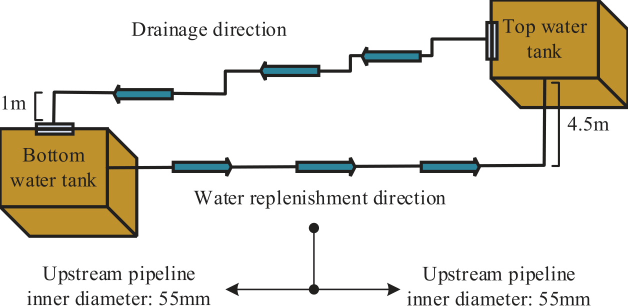
Table 1.
Test system.
Table 2.
Device Information.
Key Node Analysis
In practical engineering, the length of the tail pipe varies slightly, and the diameter of the suspension pipe and the riser pipe will be designed according to the requirements of the specifications. However, there is a lack of relevant verification methods for the length of suspension pipes. Considering the large span of the building, the suspension pipe can be laid without slope, and increasing the SPL can reduce the number of drainage risers and material consumption [26-28]. However, an increase in the SPL will also increase the system’s resistance along the way, reduce the maximum displacement (MD), and increase the siphon start time (SST) and the risk of overflow. Therefore, a reasonable SPL is crucial for optimizing the drainage system [29- 31].
The goal of this study is to develop a method for verifying the length of suspended pipes in a single bucket SDS. This is because the SPL has a significant impact on the startup time, which is very important in engineering practice. The length of the tail pipe always does not change significantly during the design process, and the verification method of the tail pipe length has a significant impact on the efficiency and stability of the system. Generally speaking, when designing an SDS, there is a tendency to choose longer suspension pipes. This can save space, avoid damaging the appearance and internal space of the building, reduce the number of components, and reduce material costs. However, as the SPL increases, the frictional resistance of the system also increases. This can lead to a decrease in the maximum drainage capacity of the system, an extension of the SST, and even the risk of gutter overflow. To solve this problem, this study takes the starting time of the siphon and the MD of the system as two limiting conditions and, through in-depth theoretical analysis and numerical calculation, attempts to develop a verification method for the SPL. The expectation is to help engineers more accurately determine the optimal SPL through this method and improve the performance of the SDS. The parameter variation range of the SDS is shown in Table 3.
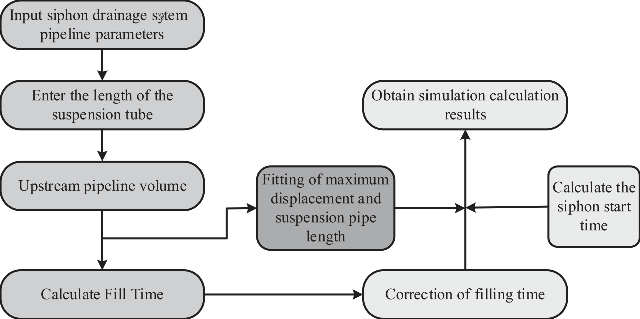
This study focuses on the study of the start time of siphons. The SST is a system dynamic state indicator that is independent of flow advancement. When the building’s height is determined, the power level of the siphon system is also determined accordingly. Therefore, if the frictional resistance of the system can be determined, the MD can be calculated. When developing a method for verifying the length of suspension pipes, an idealized analysis method was adopted. It assumes that the volume of the upstream pipeline is enriched with a smaller flow rate. As the water flow reaches the boundary points of the upper and lower pipelines, the system immediately reaches the maximum flow rate of the siphon. By setting the filling time and calculating the volume of the upstream pipeline filled, a method that is easy to understand and highly accurate can be used to estimate the SST. For different suspension pipe lengths, a correction coefficient can be obtained to determine the starting siphon time. The calculation is shown in Fig. 4.
The fitting relationship between the MD Q of the siphon and the SPL L2 is shown in formula (15).
Table 3.
Parameter variation range of SDS.
The calculation method for filling time is shown in formula (16).
In formula (16), V represents the volume of the upstream pipeline. The method for correcting the filling time is shown in formula (17).
In formula (17), α and β respectively represent correction coefficients.
Performance Simulation Analysis of Single Bucket Rainwater SDS
This study mainly explored the performance of a single bucket rainwater SDS and analyzed it through experiments and simulations. In the critical node analysis section, the study discussed in detail the effects of factors such as water replenishment, pressure difference, drainage, and pipeline flow rate on system performance.
Analysis of Test Results
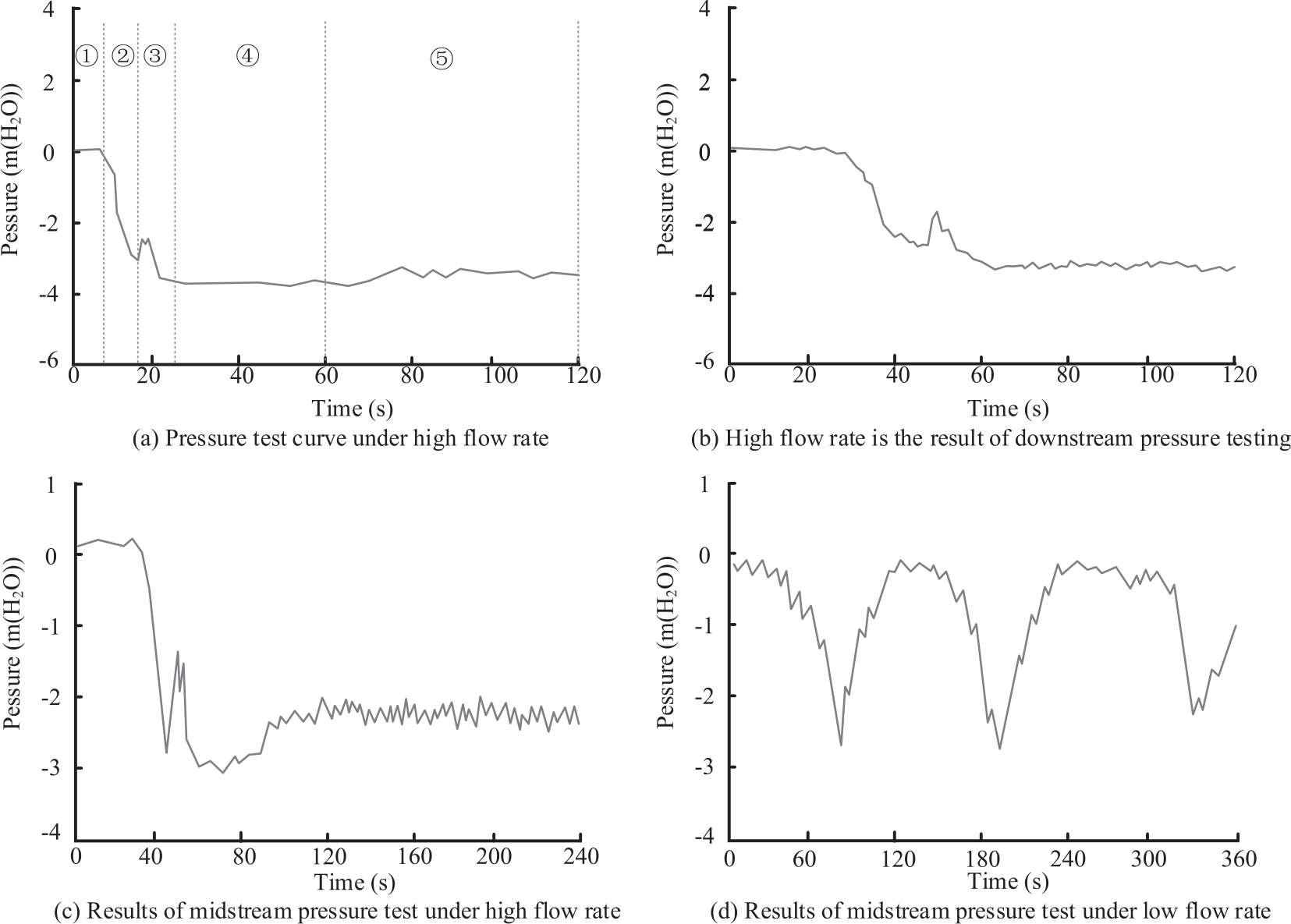
In the flow, A, B, C, and D correspond to different stages of pressure change at measuring point 3 downstream of the suspended pipe, including the zero pressure section, pressure drop section, sudden increase section, and stable section. The study observed the pressure changes under two high flow operating conditions, as shown in Fig. 5.
As shown in Fig. 5, during the flow process, ①, ②, ③, and ④ correspond to different stages of pressure change at measuring point 3 downstream of the suspended pipe, including the zero pressure section, pressure drop section, sudden increase section, and stable section. The study observed the pressure changes under two high flow operating conditions. As a large amount of residual air passes the measuring point, the pressure at the measuring point suddenly increases during the continuous decrease. At this point, the flow pattern with intermittent small bubbles does not show this sudden increase, but instead, the pressure decreases throughout the entire process to a stable stage. After the formation of a full siphon pipe, the system will maintain a maximum flow rate for drainage for a while, during which the pressure will remain at the maximum negative pressure state. If the inflow exceeds the drainage capacity, the system will remain in this state, and correspondingly, the water level in the gutter will also remain stable or continue to rise. On the contrary, if the water inflow is lower than the drainage amount, the water level in the gutter will decrease to a certain height. At this point, the system will start to inhale gas, causing the pressure to rise to a stable state. At this time, the flow state in the pipe will change into bubble flow, similar to the ③ ‘process. However, due to the large flow rate, the water filling rate in the pipe is still high, so the changes in various parameters of the system compared to the siphon flow state are very small. In addition, it can be found that even with a large flow rate, as long as a certain water filling rate is maintained, the changes in various parameters of the system are relatively small. This also proves that in the siphon operation, it is necessary to control the water inflow and drainage and maintain the water filling rate in the pipe. This can, to some extent, maintain stability, reduce the amplitude of parameter changes, and improve the controllability of the system.
Simulated Comparative Analysis
The simulation comparative analysis study conducted an in-depth comparative analysis of experimental and theoretical values for the resistance loss coefficient along the route. This comparative analysis not only helps to further understand the connotation of this important coefficient, but also helps to improve the accuracy of its application, as shown in Table 4.
As shown in Table 4, the direct test value of the average water replenishment is 45.52 m³/h. The calculated value is 46.59 m³/h. This small difference shows that the actual collected data is very close to the predicted results of the theoretical model, which reflects the accuracy of the model. However, this also means that research needs to maintain high accuracy in implementing and monitoring the replenishment process, as this may have an impact on subsequent parameters. The pressure difference between upstream and downstream testing is another important factor. The difference between experimental data of 0.612 m H2O and theoretical data of 0.60 m H2O is not significant. Similarly, the proximity of this data emphasizes the high consistency between experimental conditions and theoretical settings, which is conducive to ensuring accurate calculation of the resistance loss coefficient along the way. In drainage pipelines, displacement and pipeline velocity are key parameters that affect the coefficient of resistance loss along the pipeline. There is a subtle difference between the measured and theoretical calculation results, such as the measured displacement of 49.52 m³/h and the calculated value of 50.35 m³/h. The measured and calculated values of pipeline flow velocity of 2.57 m/s and 2.59 m/s are 1.68% and 0.77%, respectively. These all indicate that research should carefully examine and control these parameters. This not only allows the experimental results to tend toward theoretical predictions, but also helps optimize the process. Through the overall analysis, although there are slight differences between the measured values and the theoretical calculation values, these differences are within an acceptable range, all less than 2.35%. This high degree of consistency further confirms the accuracy of the theoretical model and the actual experimental settings studied. The comparison between simulation and experimental results under high flow conditions is shown in Fig. 6.
As shown in Fig. 6, a set of experimental results were compared with a set of numerical simulation results. In the comparative operating conditions, the water replenishment amount for numerical simulation was set at 15 L/S, while the average water replenishment amount for the experiment was 13.3 L/S. There is a certain difference between the amount of water replenished by numerical simulation and the average amount of water replenished by experiments. However, the numerical simulation results and experimental results have similar characteristics in the curve development trend. Specifically, the relative error between the SST of the numerical simulation and the experimental data is only -7.9%. Although there is some error, this result indicates that numerical simulation is quite accurate in predicting the start time of siphons. This verifies the effectiveness of numerical simulation methods in the study of SST. Next, the calculated MD of the numerical simulation is 16.12 L/S, while the average MD of the experiment is 14.4 L/S, with a relative error of 11.9%. Despite certain errors, important insights can still be drawn from them. Although numerical simulation methods may have some deviations in predicting the MD of a siphon system, they can generally reveal its changing trend. In summary, although numerical simulation methods may not be able to accurately simulate the actual siphoning process, their predicted trends are consistent with experimental data trends. In the process of studying the effectiveness of an SDS, numerical calculations and analysis were conducted to consider the impact of multiple factors in the system structure on the SST. It was found that changes in the values of each factor have a direct impact on the SST, as shown in Table 5.
Table 4.
Parameter variation range of SDS.
As shown in Table 5, the length of the tailpipe has a significant impact on the siphon time. The tailpipe length increased from 0.7 m to 1.1 m, and the SST increased from 7.38 seconds to 8.21 seconds, with an average sensitivity factor of -0.342. This indicates that an increase in tailpipe length leads to an increase in siphon time, indicating its importance in the system. Similarly, the increase in the SPL from 7 m to 11 m also led to a significant increase in the start time of the siphon, from 8.29 seconds to 9.12 seconds, with an average sensitivity factor of 0.499. This once again proves the impact of the increase in system length on the siphon time. The length of the riser increased from 11.5 m to 15.5 m, and the SST increased from 6.98 seconds to 7.81 seconds, with an average sensitivity factor of 0.062. Relatively speaking, the impact of riser length is relatively small, but it still proves a positive correlation between siphon time and system length. In addition, the diameter of suspension pipes and risers is also a factor that cannot be ignored. The diameter of the suspended pipe increased from 64.2 mm to 68.2 mm, causing the SST to increase from 4.92 seconds to 5.75 seconds, with an average sensitivity factor of 0.400. This indicates that the growth in pipe diameter results in a growth in the start time of the siphon. The situation of the riser is also the same. When the diameter of the riser increases from 76.3 mm to 80.3 mm, the SST increases from 5.97 seconds to 6.79 seconds, with an average sensitivity factor of 0.451. This proves that an increase in pipe diameter will prolong the start time of the siphon. Overall, an increase in the length or diameter of tailpipes, suspension pipes, or risers can lead to an increase in the start-up time of siphons. Although the degree of impact varies, the overall trend is going in the same direction. This indicates that when designing an SDS, the length and diameter of the system should be considered to reduce the SST and improve drainage efficiency. Meanwhile, the higher the sensitivity factor number, the more significant the influence of this factor on the SST. Understanding these is crucial for understanding and optimizing this system.
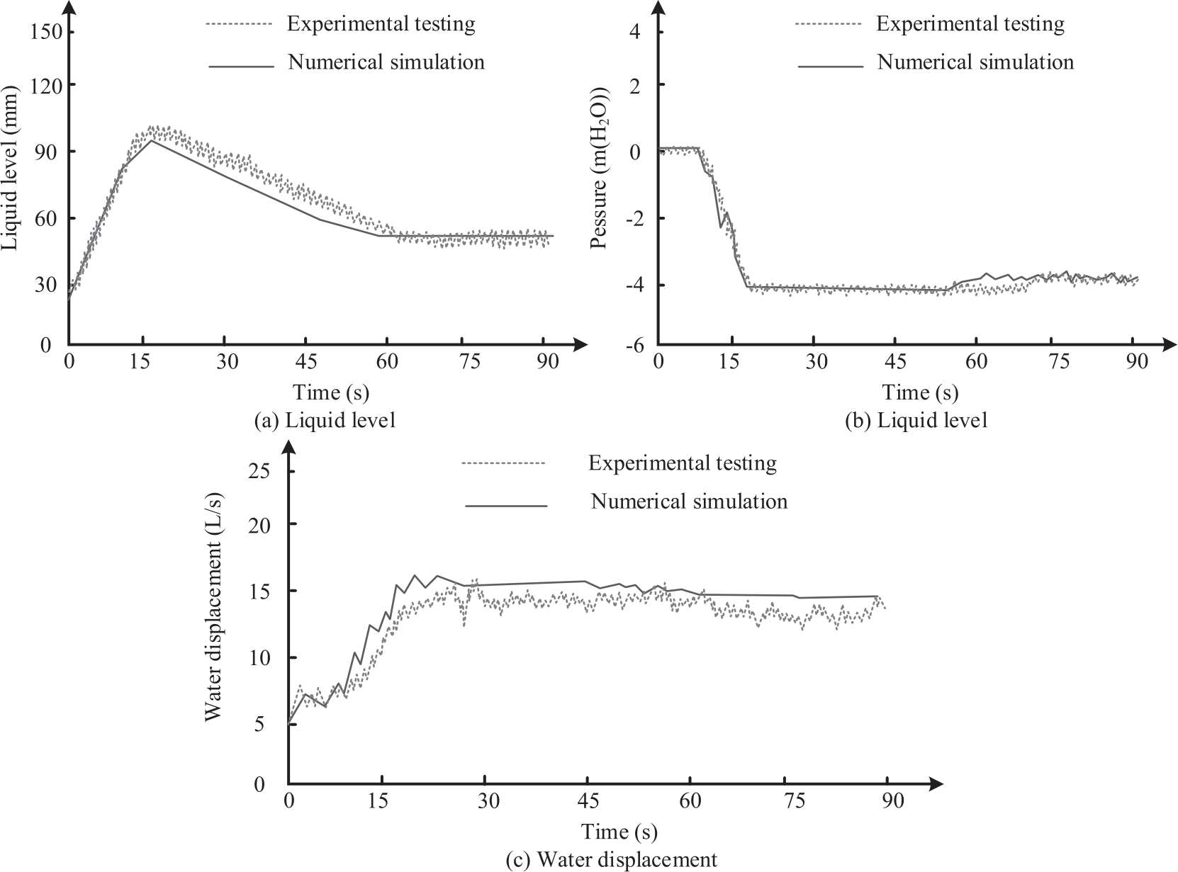
Table 5.
The influence of different factors on the start-up time of siphons.
Key Node Analysis
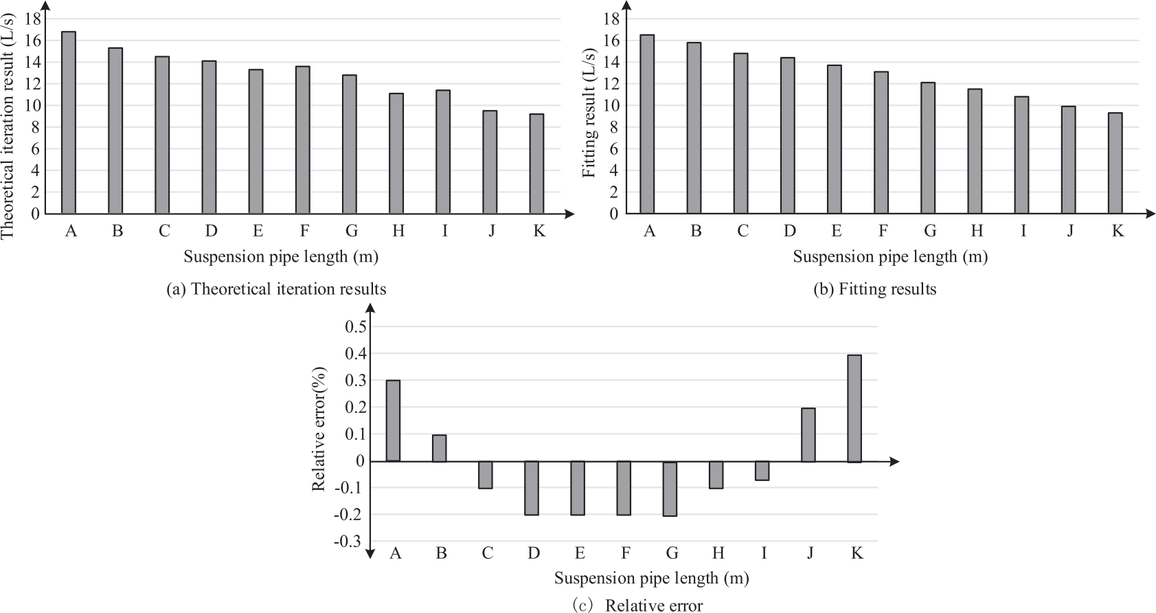
The study first analyzes the differences between model fitting and theoretical calculation results using the form of comparative error, as shown in Fig. 7.
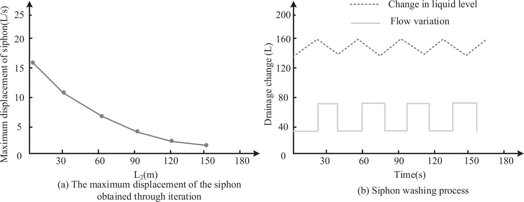
In Fig. 7, A~K are the key nodes of the single bucket siphon system, representing the top horizontal pipe, threaded rod, rainwater riser, suspension pipe clamp, rainwater bucket base, disc, square steel connector, steel pipe guide rail, square steel plate, grille top cover, and rainwater collection well. As shown in Fig. 7, the calculation results of the two are very close in most cases, although the variation range of the SPL and the flow rate is large. This phenomenon is numerically reflected in the range of relative error, ranging from 0.1% to 0.9%, but overall it is relatively small. Taking the case of a suspended pipe length of 5.7 meters as an example, the theoretical iteration result is 16.8 L/S, while the fitting formula result is 16.5 L/S. Although there is a slight difference in quantity between the two, the relative error is only 0.3%. This can be seen as the results of the two types of calculation methods being quite consistent. Similar situations also occur in other suspension pipe lengths. For example, when the SPL is 69.1 meters, the principle iteration result is 11.4 L/S, while the fitting formula result is 10.8 L/S, with a relative error of -0.07%. This once again proves that iterative calculation and fitting formulas have similar effects. It should be noted that, in some cases, the relative error is even close to 0. For example, when the SPL is 14.6 meters, the theoretical iteration result is 14.5 L/S, the fitting formula result is 14.8 L/S, and the relative error is -0.1%. This means that at this length, the two calculation methods are almost identical. The siphon drainage process is shown in Fig. 8.
As shown in Fig. 8, when the water slowly fills the upstream pipe and reaches the boundary point in the upstream and downstream of the pipeline, a significant change can be observed. At this point, the system quickly reached the maximum flow rate of the siphon, causing the gutter level to drop more rapidly. As the liquid level in the gutter decreases, when it reaches a certain level, the flow rate of the system will decrease again. The optimized table data is shown above. The following is a comparative analysis of the calculation results of the SST and the diameter of the suspension pipe, as shown in Table 6.
As shown in Table 6, for smaller suspension pipe lengths, there is a significant error between the simplified formula calculation results and the numerical calculation results. As the SPL increases, the calculation results of the simplified formula tend to be consistent with the numerical calculation results. When the SPL is 4.8 meters, the numerical calculation result of the SST is 6.4 seconds. The simplified formula results in 6.9 seconds, with a relative error of 5.65%. When the SPL is 9.7 meters, the numerical calculation result of the SST is 9.8 seconds. The simplified formula results in 9.6 seconds, with a relative error reduction of -2.14%. As the SPL increases, it is found that the simplified formula calculation results are closer to the numerical calculation results. For example, when the SPL is 39.8 meters, the numerical calculation result of the SST is 31.9 seconds. The simplified formula calculates a result of 30.8 seconds, with a relative error of only -3.56%. Through comparison, there is a certain relationship between the start time of the siphon and the SPL, and the simplified formula has slightly lower accuracy when the SPL is small. As the SPL increases, the accuracy gradually improves. In summary, although the simplified formula may have some errors in smaller suspension pipe lengths, it still has high accuracy in most cases. Considering the ease of operation and practicality of the simplified formula, this study can use the simplified formula as a method for calculating the SST. Meanwhile, to more accurately predict the start time of siphons, numerical calculation methods can be selected based on different projects and actual needs. On the ground of the calculated SPL, V, i.e., the volume of the upstream pipeline, Q, the numerical simulation results of the converted drainage flow rate of 0.6 times, filling time, and SST can be analyzed in Table 7.
Table 6.
Comparison of Calculation results between SST and suspension pipe diameter.
Table 7.
Analysis of SST.
As shown in Table 7, the first is the effect of the length of the suspended pipe on the volume (V) of the upstream pipeline. As the length of the suspended pipe increases, the upstream pipeline volume (V) also shows an increasing trend. For example, comparing the upstream pipeline volume of 30.02 liters with a suspended pipe length of 4.57 meters and the upstream pipeline volume of 264.50 liters with a suspended pipe length of 49.57 meters, the study can clearly see this change. This means that longer suspension pipes can accommodate larger upstream water bodies, which helps improve the system’s processing capacity. Secondly, the drainage flow rate (Q) shows a decreasing trend as the SPL continues to increase. As shown in the table, when the SPL is 4.57 meters, the Q value is 9.78 L/S. But when the SPL increased to 99.54 meters, the Q value decreased to 5.52 L/S. This reflects that as the SPL increases, the drainage pressure of the system will relatively decrease, which helps to protect downstream equipment or structures. The filling time (T) and SST both show a significant upward trend as the length of the suspension tube increases. The filling time increased from 3.07 seconds when the suspension tube length was 4.57 meters to 166.45 seconds when the suspension tube length was 149.78 meters. The same is true for the SST, which increased from 6.62 seconds when the suspension pipe length was 4.57 meters to 150.28 seconds when the suspension pipe length was 149.78 meters. This means that as the SPL increases, the time required for system startup will become longer, and this change will affect the operational efficiency of the system. Through the comparison and analysis of these data, it is found that the length of the suspended pipe has a certain impact on the volume of the upstream pipeline, drainage flow rate, filling time, and SST. Therefore, in actual engineering design, it is necessary to select the most suitable length of suspension pipes based on specific needs and multiple considerations such as terrain and topography. This is to achieve higher engineering efficiency and safety. This also demonstrates the necessity of conducting such numerical simulations. It can help engineers evaluate the impact of different designs on system performance and provide a basis for engineering decision-making.
Conclusion
To address the performance of a single bucket rainwater SDS and the impact of the SPL, this study adopted a design of simulated operation models and actual size models. It utilizes a combined strategy to test the various performances of the system. It is verified through a comparison between experiments and practical applications. The results showcase that the pressure at the measuring point continues to decrease under high flow operating conditions. The reason for the sudden increase is that lots of residual air passes the measuring point, and the system remains in a maximum flow drainage state. In terms of the relationship between SST and various factors, there is a positive correlation between tail pipe length SST, suspension pipe length SST, and riser length SST. When the length of the tail pipe increases from 0.7 m to 1.1 m, the SST increases from 7.38 s to 8.21 s. When the SPL increases from 7 m to 11 m, the SST increases from 8.29 s to 9.12 s. When the length of the riser increases from 11.5 m to 15.5 m, the SST increases from 6.98 s to 7.81 s. Therefore, the start-up time and MD of the siphon are key factors in the siphon’s drainage performance. These two parameters are also influenced by the height of the building, the system resistance along the way, and the SPL. Therefore, it is necessary to design an effective verification method to determine the optimal suspension pipe length to optimize the performance of the SDS. It has important research value and practical significance. At the same time, it was found in the experiment that the structure of the siphon rainwater bucket has a significant impact on the drainage effect, and the rainwater bucket structure used in the study is too simple. When completing a siphon, a large amount of air is sucked in, making it difficult to make up the water conversion between gravity flow and siphon flow. Further optimization of the rainwater bucket structure can be carried out in future research to enhance its air blocking effect. At the same time, actual rainfall is dynamic and varies over time. Therefore, further research can be conducted to explore the changes in parameters and start-up time of the siphon drainage system under changes in water replenishment and to explore the possibility of applying the multi bucket system under this concept.

