

Introduction
China’s 14th Five-Year Plan (2021-2025) for Modern Logistics Development, issued by the State Council and the General Office on May 2022, emphasizes the strategic importance of the logistics industry in upgrading value chains, building supply chains, promoting high-quality development (HQD), and establishing modern economic systems. The logistics industry’s HQD is thus an essential component of economic HQD in China. Therefore, as China transitions from a rapid growth economy to HQD economy, the logistics industry, which is closely linked to this transition, has also entered a key phase of improving quality and efficiency from an extensive development mode. However, resource allocation of China’s logistics industry remains unreasonable, with high levels of investment and energy consumption, low efficiency, and environmental degradation emerging as prominent issues [1].
According to the China Statistical Yearbook (2007, 2021), the energy consumption of the transportation, storage, and postal industries in China has risen dramatically from 186 million tons of standard coal in 2006 to 413 million tons of standard coal in 2020, with its share of total energy consumption increasing from 7.5% to over 9.0%. To achieve green sustainable development, the logistics industry’s HQD should simultaneously consider enhancing economic and environmental benefits [2]. Green total factor productivity (GTFP) is a key indicator for measuring economic and environmental performance [3]. Therefore, research on the logistics industry’s GTFP (LGTFP) is crucial for improving the quality of logistics development and realizing long-term sustainability.
Improvements in GTFP are affected by several factors, such as the economic development level [4], technological innovation (TI) [5, 6], environmental regulation (ER) [7, 8], infrastructure level [9], and energy structure [10]. Among these influencing factors, TI is a pivotal force that drives sustainable and healthy economic development [11] and regional green development [12]. Simultaneously, to reduce pollution, improve the ecological environment, and meet China’s goal of peak carbon emissions, relevant sectors have introduced a range of ER measures. These environmental regulatory measures have impacted the level of TI and improvements in GTFP [13].
The relations among TI, ER, and the GTFP in various regions and industries in China has become a hot topic for scholars [5, 14-16]; however, few studies have examined the relations among TI, ERs, and LGTFP. Existing literature has only studied the influence of a single factor, TI [17] or ERs [18] on LGTFP. Few studies have incorporated TI, ERs, and the LGTFP into the same research framework. Thus, the following questions warrants further research: Can TI enhance the LGTFP? Does the relation between TI and LGTFP vary with the level of ER? How does the interplay of TI and ER impact LGTFP?
This study addresses this research void by examining TI’s influence on LGTFP and the moderating impact of ER on this relation. In the 11th Five-Year Plan (2006- 2010), the government for the first time clearly proposed that “energy conservation and emission reduction” should be a binding indicator for environmental protection and linked to performance evaluation. This indicates that ER has become a mandatory constraint indicator, which has an important impact on the formulation and implementation of ER-related policies. The year 2020 is the end of the 13th Five-Year Plan (2016-2020). To this end, we selected data from 30 Chinese provinces during 2006-2020, and calculated the LGTFP, which is used as the dependent variable in our analysis. Clarifying the internal relations among TI, ER, and LGTFP holds both theoretic and practical value for enriching the theoretical mechanism of the logistics industry’s HQD and formulating more reasonable ER and ecological protection policies.
The possible marginal contributions of our study are: (1) unlike previous studies that used traditional data envelopment analysis (DEA) or slack-based measure (SBM) to measure LGTFP, we used the Epsilon-based measure and global Malmquist-Luenberger index (EBM-GML) to evaluate changes in LGTFP. (2) Studies in the literature mostly considered the influence of a single factor – TI or ER– on LGTFP. In our study, TI, ER and LGTFP are integrated into the same research framework, and the internal influence relations among them are analyzed. (3) Earlier studies mostly used conventional econometric model approaches, but ignored the cross-spatial correlation and spillover effects of LGTFP, TI, and ER. We construct a dynamic spatial Durbin model (SDM) for analysis, which can prevent the bias arise form ignoring geospatial factors.
Literature Review
Method to Measurement GTFP
Methods of measuring productivity could be categorized into two types: parametric and non-parametric. The former primarily includes the stochastic frontier method and the parametric linear programming method, while the latter primarily includes the DEA method and Malmquist index. Parametric methods require a specific functional form and have strict assumptions regarding function distribution, which could result in larger errors if these assumptions are not met. Non-parametric methods are widely used to measure GTFP because they do not need assumptions, have lower requirements for data dimension indicators and sample size, and can handle multiple input-output variables directly [19]. For example, Tian and Lin [20] and Li and Lin [21] used the Malmquist-Luenberger (ML) productivity index based on the directional distance function (DDF) model to evaluate China’s industrial and cities’ GTFP. However, the DDF model ignores slack variables and could overestimate efficiency. Therefore, Tone [22] put forth an SBM model that considers slack variables. Liang et al. [23] and Zhou et al. [24] utilized the SBM-ML and SBM-DDF-LPI, respectively, to estimate the LGTFP in Jiangsu Province and other provinces in China and studied the environment’s influence on it. However, the SBM model cannot measure input-output indicators that contain both radial and non-radial relations. To solve this issue, Tone and Tsutsui [25] developed a hybrid model known as the EBM model, which can handle both radial and non-radial input-output indicators simultaneously. This model compensates for some of the defects of the SBM model and makes the measurement results more accurate and reliable. Additionally, because the ML index could yield infeasible solutions, Oh [26] introduced the GML productivity index, which overcomes the infeasible solutions problem and meets the circularity requirements, making the results more accurate and comparable. This study therefore selects the EBM-GML index to calculate the LGTFP, as it overcomes issues related to radial and non-radial inputs and outputs while avoiding non-solutions and non-circulation problems [27, 28].
Influence of TI on GTFP and its Spatial Spillover Effects
Influence of TI on GTFP
As China is increasing its focus on environmental quality, the impact of TI in decreasing carbon emissions and enhancing GTFP has gradually become a research hotspot. Existing research suggests that TI has three main impacts on productivity: positive promotion, inhibition, and nonlinearity.
TI has a positive effect on productivity. TI can promote productivity by improving energy utilization efficiency [29-31], reducing energy consumption and pollutant emissions [32, 33], and improving production efficiency by optimizing factor allocation [34]. Regarding the logistics industry, Yang [35] and Jian et al. [36] claimed that TI can drive logistics industry’s transform to intensification, standardization, and intellectualization; improve its operation quality; and significantly promote the logistics industry’s HQD. Zhang et al. [37] demonstrated that TI in reverse logistics is conducive to resources recycling, and enhances GTFP by enhancing resource utilization efficiency. Additionally, Bag et al. [38] and Mastos et al. [39] proposed that the integration of new technologies, such as big data and artificial intelligence, can facilitate the efficient allocate of resources in the logistics industry and improve business processes. They play a vital role in operational management and productivity improvements in the logistics industry.
Further, the influence of TI on productivity is either hindered or nonlinear. Liu et al. [40] found that TI significantly enhanced ecological efficiency in the Poyang Lake urban agglomeration; however, it had an energy-rebound effect in the Wuhan metropolitan area, which escalated its energy depletion and inhibited the enhancement of GTFP. Brännlund et al. [41] also demonstrated that TI could increase energy demand, which could lead to an energy-rebound effect, resulting in higher emissions of CO2, SO2 and other polluting gases. Liang et al. [8] demonstrated that the logistics industry’s TI can reduce its CO2 emissions by increasing the use of green packaging, adopting new energy trucks, and reducing the rate of driving empty vehicles. However, the logistics industry’s TI has a rebound effect on CO2 emissions. Thus, the impact of TI on CO2 emissions is “U-shaped”.
Spatial Spillover Effect of TI
As industries become increasingly interconnected, the spillover effect of technology among industries becomes increasingly significant [42]. Therefore, the spatial spillovers of TI have received increasing attention in recent years. Some scholars believe that TI has significant positive spatial spillovers that can reduce carbon emissions in adjacent regions and improve GTFP. Jiao et al. [42] have demonstrated that the spillover effect of TI through industrial linkages has a more pronounced effect on reducing carbon intensity. Utilizing the SDM and China’s city-level panel data during 2003-2017, Sun et al. [43] also demonstrated that the spillover effect of TI notably decreased neighboring cities’ carbon intensity; however, other scholars concluded that TI has negative or nonlinear spatial spillovers. Wang et al. [44] explored the effect of TI on China’s GTFP and found that it had significant positive and negative impacts on the GTFP of local’s and neighbors’ respectively. However, Xiao et al. [45] concluded that the impact of agricultural technical advancements on agricultural GTFP on local and neighboring areas were “inverted U-shaped” and “U-shaped”, respectively, during 1998-2019.
In the areas of transportation and logistics, the vertical spillover effect of transportation emission reduction technique is even higher than the effect of the technology stock itself [42]. Therefore, green transportation emission reduction technology should be vigorously pursued. Moreover, Yang et al. [6] showed that research and development investment positively impact the transportation industry’s GTFP during 2005- 2017, whereas inter-provincial technology spillover negatively impacted the transportation industry’s GTFP. Liang et al. [8] also found that the logistics industry’s TI has spatial spillovers, which could intensify the rebound effect of carbon emissions in adjacent regions, thus negatively affecting LGTFP in neighboring areas.
ER, TI, and GTFP
ER and TI
There is no consensus regarding the relations between ERs and TI. Johnstone et al. [46] assessed the effect of ER strictness on TI based on surveys and patent statistics in 77 countries during 2001-2007 and found that strict ER positively impacted enterprise innovation. Song et al. [34] focused on resource-based enterprises data and examined the effect of ER on TI in manufacturing industries using the TI compensation theory of ER and discovered that ER can stimulate green TI in resource-based manufacturing industries. Based on vehicle specification data, Kiso [47] compared and analyzed the impact of ERs on vehicle fuel economy and found that ERs can promote TI in vehicle fuel efficiency and improve vehicle fuel economy by 3%-5%. However, Shi et al. [48] showed that ER policies significantly inhibit enterprise innovation, with their suppressive impact increasing over time. Zhou et al. [49] identified an “inverted U-shaped” relation between formal ERs and innovation in China’s Yangtze River Delta region.
ER and GTFP
An overview of the literature shows that ERs has three main influences on GTFP: promoting, inhibiting, and nonlinear. Ai et al. [50] demonstrated that ER can improve allocation efficiency of factors and positively impacts industrial enterprises’ GTFP. Some studies demonstrated a positive effect of ER on GTFP in industries [51, 52] and cities [23] in China. However, Wu and You [53] and Xia et al. [54] concluded that command-control ERs markedly inhibit the improvement of local GTFP. More research showed that the relations between ERs and GTFP is nonlinear. For instance, Wang and Shen [55] examined the effect of ER on industrial environmental productivity in China and concluded that the impact is “inverted U-shaped”. Wang et al. [56] showed that ER has a threshold level, and its influence on GTFP is “inverted U-shaped”. However, Qiu et al. [57] reached an opposite conclusion: that ER has a “U-shaped” impact on GTFP. Li and Li [15] found that the effect of ER on GTFP in moderately and heavily polluting manufacturing industries is “U-shaped”, whereas the impact on GTFP in lightly polluting manufacturing industries is non-significant. According to Liang et al. [23] and Pei and Mu [58], there is also an inflection point or threshold effect associated with ER’s impact on LGTFP.
Moderating Effect of ER
Some studies have shown that ERs moderate the relation between TI and productivity. Chan et al. [59] concluded that green product innovation and development ability are key to enhancing corporate competitiveness, which positively impacts enterprise performance, and that ERs have a moderating effect on this impact. Pan et al. [60] found that TI improves energy efficiency, and that this influence is affected by ERs. Jin et al. [14] found that while TI alone does not significantly improve industrial water resources’ GTFP, but its interaction with ER significantly enhances industrial water resources’ GTFP. This suggests that ERs moderate the effect of TI on GTFP. Kong [61] also indicated that both command-control and market-incentive ERs can effectively moderate the relation between innovation capability and GTFP.
By reviewing the available literature, we discovered that, first, most published studies utilized traditional DEA or SBM models to assess GTFP, but none could deal with input-output indexes containing both radial and non-radial relations. EBM compensates for the defects in the above models, and the GML index is comparable and transitive. Therefore, the EBM-GML model was selected to evaluate changes in LGTFP, resulting in more accurate and reliable measurements. Second, few studies examined relations among TI, ERs, and LGTFP, and most either considered the impact of a single factor of TI or ER on LGTFP. Few studies have simultaneously incorporated TI, ERs, and the LGTFP into the same research framework. It is crucial to clarify the internal relations among TI, ER, and the LGTFP to enrich the theoretical mechanism of the logistics industry’s HQD. Third, most existing studies used traditional econometric models to study relations among TI, ER, and GTFP but did not consider objective spatial factors and rarely considered spatial spillover effects.
Consequently, we employ the EBM-GML index to assess changes in LGTFP in 30 provinces in China (Xizang, Hong Kong, Macau, and Taiwan were excluded owing to missing data) and adopts dynamic SDM to perform a thorough analysis of relations among TI, ER, and LGTFP. This study enriches the theoretical mechanism of LGTFP; practically, this could help the government formulate more reasonable ERs and ecological protection policies. Therefore, our study holds notable theoretical and practical implications for logistics industry’s HQD.
The Influence Mechanisms and Hypotheses of TI, ER, and LGTFP
Influence Mechanism of TI on LGTFP
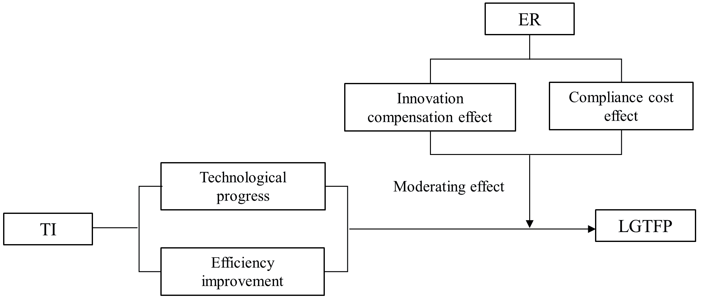
The theory of endogenous economic growth and innovation believes that TI can promote the improvement of GTFP through endogenous effects of technological progress and efficiency improvement. The logistics industry’s TI can promote innovation in its technological equipment, accelerate its automation and intelligence [35], promote the progress of production technology, improve the service quality of the logistics industry, reduce service costs, and improve its production efficiency. Concurrently, the product and process innovation of enterprises will optimize the combination of production factors, improve the efficiency of resource allocation, reduce energy consumption and pollutant emissions, and ultimately enhance LGTFP.
From the above literature review, the logistics industry’s TI can not only improve local LGTFP but also have an impact on neighboring areas. Regions with TI advantages often have a better economic foundation and research and development (R&D) environment. These advantages will draw in workforce, financial, and other related resources from neighboring areas through the “siphon effect”—resulting in the loss of resources, capital, and technology in neighboring areas, thereby reducing their LGTFP [62]. Therefore, TI can have a negative spatial spillover effect on LGTFP in surrounding areas through the “siphon effect”.
Based on the analysis of the impact mechanism of TI on LGTFP and its spatial spillover effects, we formulate the first hypothesis:
Hypothesis 1: TI has a positive and direct effect on LGTFP but negative spatial spillovers on neighboring areas’ LGTFP.
Influence Mechanism of ER on TI and LGTFP
The influence of ER on TI and LGTFP is mainly through two aspects. First, ER affects TI and LGTFP by causing changes in enterprise costs; that is, the “compliance cost” effect. ER will increase the cost of pollution control and increase the cost of enterprises. Driven by the principle of profit maximization, enterprises will compensate for the cost of investment in environmental governance by reducing TI investment such as R&D, which will adversely affect TI and LGTFP [63]. Second, ER improves TI and promotes LGTFP through the “innovation compensation” effect. The “innovation compensation” effect mainly means that appropriate ER policies can encourage enterprises to perform TI, explore green production methods with competitive advantages, balance environmental and economic performance, improve enterprise operating conditions, increase profits, make up for the increased cost owing pollution control, and ultimately enhance LGTFP. Therefore, the impact of ER on TI and LGTFP is a game between “innovation compensation” and “compliance cost” [64]. The influence of TI on LGTFP will vary with the intensity of ER; that is, ER most probably modulates the relation between TI and LGTFP in a nonlinear manner. Thus, we formulate Hypothesis 2.
Hypothesis 2: ERs play a nonlinear modulatory role in TI’s influence on LGTFP.
Research Methods, Variable Selection, and Data Sources
Research Methods
Construction of Econometric Model
The levels of TI, ER, and LGTFP within a region are influenced not only by the region’s own resources, economic level, and other factors but also those of surrounding cities. Further, the relevant literature shows that TI’s influence on GTFP exhibits spatial spillovers [16, 44]. This study discusses the relations among these three factors through a spatial econometric perspective. In the spatial model setting, the omission of the spatial lag term of the dependent variable or independent variable will cause bias in the model setting, resulting in biased and inconsistent estimators [65]. The SDM considers the spatial lag terms of both independent and dependent variables, and there is no need to add a priori constraint to the spatial interaction of potential independent variables [66]. Therefore, we constructed SDM to study the relations among TI, ER and LGTFP. The test results of the model selection in 5.2 also shows that our choice is appropriate. Equation (1) represents the general form of SDM.
Where y is the dependent variable, while X represents the independent one; ρ is the spatial autoregressive coefficient; β and θ denote parameters to be estimated for X and its spatial lag item; W signifies the spatial weight matrix; and u indicates spatial disturbance term.
In addition, since GTFP changes are dynamic and continuous, current GTFP is affected by previous levels, which is easy to produce path dependence [67]. Therefore, we introduce a lagged period for the LGTFP and construct dynamic SDM. The dynamic SDM contains both spatial and time lag terms of the explained variables, which can avoid path dependence and endogeneity problems [68]. The SDM shown in Equations (2-4) are constructed based on Equation (1) to explore the relations among TI, ER, and the LGTFP to empirically test the above research hypotheses.
(2)
(3)
(4)
Table 1.
Input–output indicators of LGTFP.
Model (2) tests the direct and indirect influences of TI on LGTFP. We include the interaction term of TI and ER in Model (3) and introduce the interaction item of TI and ER squared in Model (4) to examine the nonlinear moderating effect of ER.
Selection of Spatial Weight Matrix
Owing to the absence of a unified construction standard for the spatial weight matrix and in consideration of the actual situation of the logistics industry, this study constructed an adjacent spatial weight matrix according to the methods used by Hao et al. [69] and Wu and Wang [70]. The formula is as follows:
Variable Selection and Data Sources
Dependent Variable and Data Sources
This study calculated the LGTFP using the EBM-GML index. For the specific calculation formula, refer to Deng et al [27]. Table 1 summaries the selected input-output indicators. Considering that the growth rate of the LGTFP is obtained by using the EBM-GML index, we utilized the cumulative multiplication method proposed by Chen et al. [71] and Shen et al. [72] to convert it into the actual value of the LGTFP for further analysis. Assuming that the LGTFP in the base year 2006 was 1, the resulting LGTFP after multiplication represents the years 2007-2020.
Input index selection
Capital and labor are fundamental components of production and economic activities in various industries [73], and energy consumption is a key input for the logistics industry. Therefore, for LGTFP computation, we selected capital stock, number of employees, and energy consumption as input indicators. Considering that China’s logistics industry lacks complete statistical data, so we draw on the work of Zheng et al. [74], Wang and Xin [75] and Li and Wang [2] used statistical data on the transportation, warehousing, and postal industries to represent the logistics industry.
As data on the logistics industry’s capital stock are unavailable directly, we referred Long et al. [76] and utilized the perpetual inventory method to evaluate it. The formula is,
δt signifies depreciation rate in year t, which is 9.6% in this study, Iit and Pit are fixed asset investment and its price index of the logistics industry in year t of region i, respectively. Data are reduced to a constant price based on 2006. We use the method of Zhong and Wang [77] to estimate base capital stock.
China Statistical Yearbook (2007-2021) data on transportation, warehouse, and postal employees is used to as the number of logistics employees. Following Li and Wang [2] and Long et al. [76], we selected eight energy sources (raw coal, gasoline, kerosene, diesel, fuel oil, liquefied petroleum gas, natural gas, electricity) that are more expended in logistics industry as energy inputs. Data of these sources were converted into standard coal using their energy conversion coefficients.
Selection of Output Indicators
As a production service industry, logistics industry’s expected output should be the total effect it has on service objects. However, the total effect cannot be measured scientifically. Therefore, numerous studies have adopted logistics industry’s added value as a value form to assess its expected output [78, 79]. We draw on these studies and use the logistics industry’s added value as the expected output indicator. To adjust the data to a constant 2006 price, we employed the price index of the tertiary industry’s added value.
The logistics industry’s main form of pollution is CO2 emissions. Therefore, we considered CO2 emissions as the undesired output. Combined with data availability of the logistics industry, we calculated its CO2 emissions using the “top-down” method provided by IPCC [80]. The formula is as follows:
Ei signifies the consumption of i − th energy; NVi, EFi, and OFi indicate the average low calorific value, carbon content per unit calorific value and carbon oxidation factor of i − th energy, respectively.
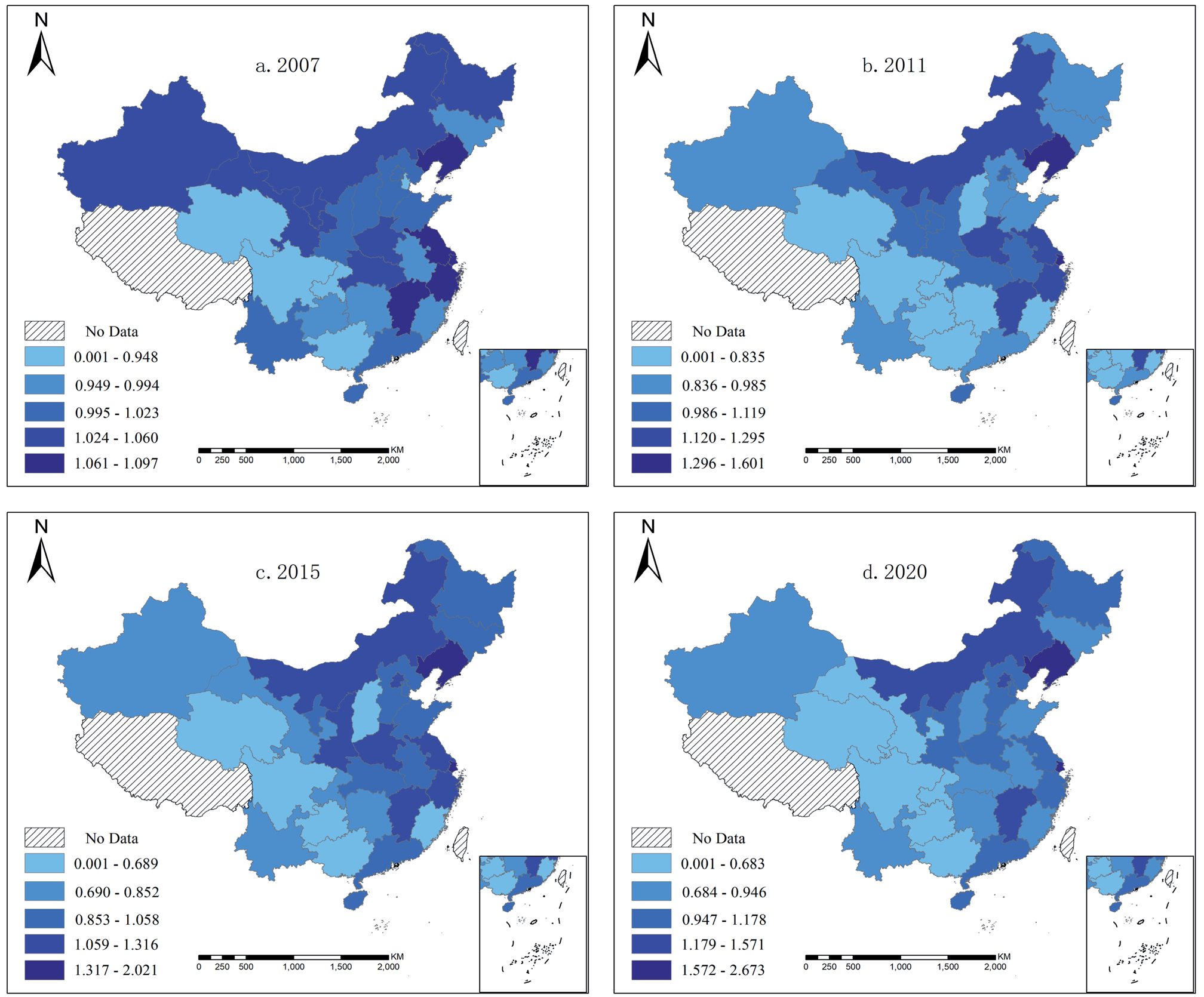
Based on the EBM-GML index, we calculated the LGTFP of 30 provinces in China during 2006-2020. We selected the productivity values of 2007, 2011, 2015, and 2020 and used ArcGIS10.2 to draw the spatial distribution evolution map of LGTFP. As demonstrated in Fig. 2, the spatial distribution of LGTFP in China gradually develops spatial clustering features. High LGTFP areas gradually became concentrated along the eastern and south-eastern coastal regions, while low LGTFP areas were primarily concentrated in the western region.
Explanatory Variables and Data Sources
Core explanatory variable: TI. Griliches [81] showed that patents are closely associated with innovation and that their authorization standards are relatively stable. Scholars often use patent data to measure innovation levels. Following Dang and Motohashi [82] and Hao et al. [69], we considered the patent invention authorization quantity per 10,000 people in the logistics industry as an indicator of TI. Data on invention patent authorization were collected from the logistics industry patent information service platform of the China Intellectual Property Office and include six categories: loading and unloading, logistics transportation, inventory technology, distribution processing, sorting, packaging and distribution systems, and logistics information technology.
Moderator variable: ER. Since there are no direct data on the level of ER, previous studies mainly measured the level of ER through data, such as pollution control investment as a percent of GDP, the sum of the three waste discharges, and the number of ERs issued by the government. Drawing on Li et al. [83] and Liu and He [84], we assessed ER by the completed investment amount of industrial pollution control per thousand yuan in the secondary industry’s value-added.
Control variable. In addition to ER and TI, LGTFP is affected by various other factors, for instance economic development level and energy structure. To reduce the result bias caused by omitting other factors, borrowing from Yang et al. [6] and Long et al. [76], we chose five indexes-economic development (ED) level, industrial structure (IS), energy structure (ES), opening-up (OP) level, and labor productivity (LP)- as control variables. Each province’s per-capita GDP indicated its level of economic development while the percentage of the tertiary sector’s added value of GDP signified its industrial structure. The level of opening-up was evaluated as foreign direct investment’s share of GDP, and energy structure was denoted as the share of electrical expenditure in total energy consumption. In addition, labor productivity of the logistics industry was measured by the ratio of its added value to the total number of employees.
All the data presented above were collected from the China Statistical Yearbook (2007-2021) and the China Energy Statistical Yearbook (2007-2021). Table 2 provides a descriptive statistical analysis of all variables and data.
Empirical analysis
Spatial Correlation Test
Examining the spatial correlation of the data is essential before constructing a spatial econometric model. Global and local spatial autocorrelation measures are often adopted for this purpose. We selected global Moran index to examine the spatial correlation of LGTFP in China during 2007-2020 using the adjacency matrix. Table 3 summarizes the measurement results, while the Moran scatter diagram is illustrated in Fig. 3.
Selection of Spatial Econometric Models
The spatial autocorrelation test demonstrated that LGTFP has a significantly positive spatial correlation. Next, we selected the model followed the analysis process recommended by Elhorst [85]. First, since the level of TI, ER and logistics industry in each province is different, we adopted the fixed effect model for spatial regression analysis. Our choice was also verified by the Hausman test results. Second, we performed Lagrange Multiplier (LM) tests, including ordinary and robust LM tests, to confirm whether there was a spatial lag and error term. The results of both tests were significant, so we could not determine which of the two models was more suitable. We therefore selected the SDM with the dual effects of spatial lag and error. Third, both Wald and likelihood ratio (LR) were significant, so SDM would not degenerate into spatial lagged and spatial error model. Based on these outcomes listed in Table 4, we determined that the SDM under fixed effects was the optimal choice.
Regression Results Analysis
The results obtained from the above variables and models are summarized in Table 5. The findings demonstrate that the spatial autoregressive coefficients of LGTFP in Models (2)-(4) were 0.1769, 0.3426 and 0.4612, respectively (all ps<0.01). This suggests that the promotion of local LGTFP can improve LGTFP in neighboring regions. The time-lag coefficients of LGTFP in the three models were 1.3745, 1.7031, and 1.7067, respectively (all ps<0.01), indicating that the positive influence of the previous period LGTFP on the current is significant. In Model (2), the regression coefficient and spatial lag coefficient of TI are 0.2116 and -0.1836, respectively (both ps<0.01). This demonstrates that TI promotes the increase of the local area’s LGTFP but inhibits the neighboring areas’ LGTFP increase. In Model (4), the interaction coefficient of TI and ER is significantly negative, whereas the interaction coefficient of TI with ER squared is significantly positive. Therefore, ER has a “U-shaped” moderating effect in the impact mechanism of TI on the LGTFP, and the regulatory effect diagram is shown in Fig. 4.
Table 3.
Global Moran index of LGTFP.
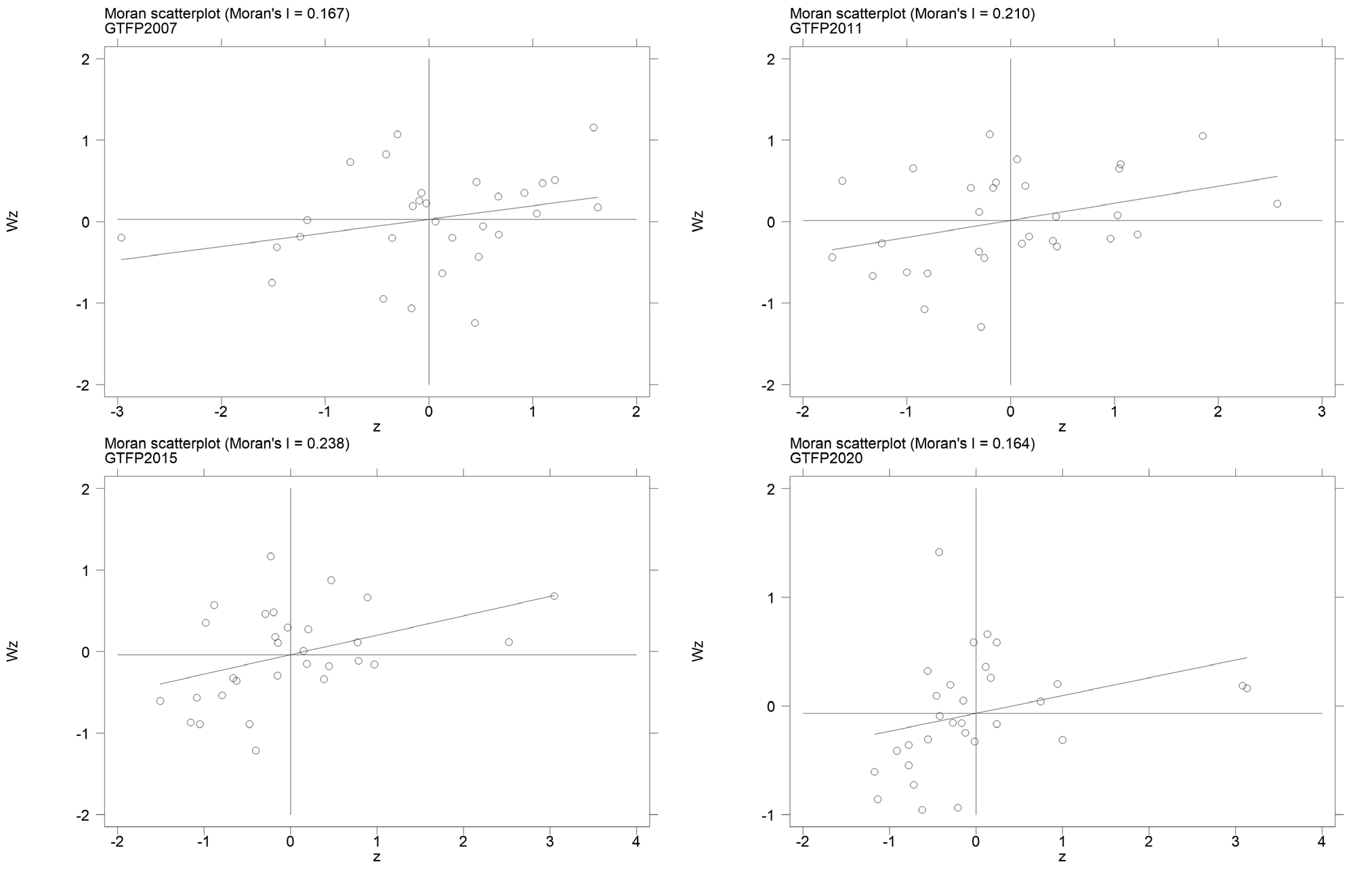
Table 4.
LM, Hausman, Wald, and LR tests.
Table 5.
SDM regression results.
Given the coefficients of exogenous variables and their spatial lag items in the SDM are not the real influences on the dependent variable; therefore, the direct and indirect effects must be calculated. Hence, effect decomposition was performed for Models (2) and (4) to calculate the direct and indirect effects. The outcomes of the effect decomposition are displayed in Tables 6 and 7.
According to Table 6, the effect decomposition of Model (2) demonstrates that the direct and indirect effect coefficients of TI on LGTFP in the short term are 0.2049 and -0.1680, respectively (both ps<0.01). This means that, in the short term, TI can boost the enhancement of local LGTFP but will have negative spatial spillovers on adjacent regions. This result confirms Hypothesis 1 and also corroborates the conclusions of Wang et al. [44] and Liang et al. [8]. There are three possible reasons for this finding. First, in the short term, TI can enhance the energy efficiencies in freight transportation and other links, reduce energy consumption and CO2 emission, and thus improve the LGTFP [8]. Second, TI promotes the demand for regional logistics and freight markets, improves the logistics industry’s distribution capacity and transportation benefits, and improves LGTFP [86]. Third, in the short term, the improvement in TI in local regions will draw in manpower, capital, and other related resources from neighboring areas, resulting in a “siphon effect” [62]. This will give rise to a loss of resources, capital and technology in neighboring areas, thereby reducing the LGTFP.
The effect coefficient of TI on local LGTFP is -0.6434 in the long-term (p<0.01). This result may appear to be contrary to our expectations, but we cannot simply conclude that TI in the logistics industry inhibits LGTFP. The energy-rebound effect could be a possible explanation. In the long run, TI will reduce energy consumption per unit of product while enhancing energy utilization efficiency and further increase the logistics industry’s energy consumption through mechanisms like substitution, income, and output effects [87]. This rebound phenomenon can give rise to a marginal increase in energy consumption and pollutant discharge, thereby reducing LGTFP. Vivanco et al. [88] also discovered that, owing to the rebound effect, TI can indirectly increase the environmental pollution of the transportation sector. This also corroborates the conclusions of Liu et al. [89], Liang et al. [8], and Liu et al. [90] – that TI in the transportation and logistics industries has a rebound effect on energy consumption and air pollution. TI has a significantly positive long-term indirect influence, indicating a significantly positive impact on LGTFP in adjacent regions. The possible reasons are twofold. First, in the long run, when TI develops to a certain level, it could produce agglomeration and a diffusion effect, drives the improvement of LGTFP in neighboring areas. Second, technical exchanges and cooperation with neighboring areas will be strengthened in long-term development, which will enhance the spillover and transformation of TI achievements and neighboring areas’ LGTFP.
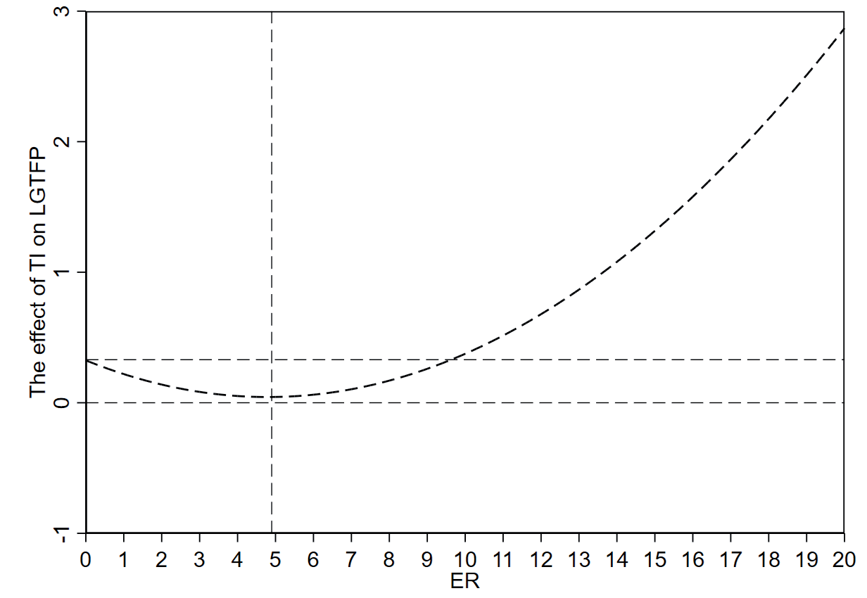
The Model (4) effect decomposition results in Table 7 reveals that, in the short term, the interaction coefficients between TI and ER and TI and ER squared are significantly negative and positive, respectively. These outcomes indicate that ER has a “U-shaped” moderating effect in the impact mechanism of TI on the LGTFP in the short term, which confirms Hypothesis 2. Weak ERs display negative regulatory roles in the impact mechanism of TI on LGTFP, and consequently weakens the positive effect of TI on the LGTFP. Strengthened ERs have positive moderating effects in the impact mechanism of TI on the LGTFP. That is, strong ERs strengthen the positive effect of TI on the LGTFP. This could be because in the short term, when the intensity of ER is weak, enterprises tend to occupy TI investment funds for pollution control. The reduction in TI funds decreases the TI capabilities of enterprises and their innovation output [91]. Therefore, the favorable influence of TI on LGTFP is suppressed. However, when the intensity of ERs is high, taking up investment in TI to passively control pollution does not achieve pollution control. Enterprises will increase their investments in pollution control and production technology innovation to enhance their level of TI and improve the level of emissions reduction and pollution control in production process. Therefore, in the short term, high-level ER facilitates the positive effect of TI on LGTFP.
Further, the indirect effect coefficient for the interaction of TI with ER square is also positive and significant (p<0.01) in the short term. This indicates that ERs have “U-shaped” modulation on the effect of TI on LGTFP in neighboring areas. Thus, ER has the same moderating effect in the effect mechanism of TI on both local and adjacent areas’ LGTFP.
In the long run, the interaction coefficients between TI and ER, and TI and ER squared are 0.2851 and -0.0299, respectively (both ps<0.01). This outcome suggests that ER plays an “inverted U-shaped” moderating role on the mechanism of TI’s influence on LGTFP. This result also confirms the Hypothesis 2 that ER plays a nonlinear regulatory role in the effect of TI on LGTFP. Weak ERs have positive modulatory roles in the influence mechanism of TI on LGTFP, meaning that the negative influence of TI on LGTFP can be alleviated when ER levels are low. However, when ER reaches a certain level, it negatively regulates the relations of TI with LGTFP; that is, the negative effect of TI on LGTFP can be exacerbated by high levels of ER. This could be because, in the long run, weak ER intensity can also promote TI to a certain extent and improve GTFP through innovation compensation and enhanced energy utilization efficiency [49]. However, weak ER intensity is not sufficient to form a strong incentive effect on TI, and the energy-rebound effect owing to TI will be low. Therefore, long-term low levels of ERs weaken the negative effect of TI on GTFP. However, long-term high ER intensity compels the logistics industry to perform TI, improve its development level, promote freight demand and energy consumption, and increase the energy-rebound effect brought by TI. Simultaneously, strict ERs could exhaust excessive financial resources in the long-term, and weaken the overall competitiveness of the industry [92], which is detrimental to the improvement of LGTFP. Therefore, higher ER intensity intensifies the negative effects of TI on the LGTFP in the long term.
In the long run, the indirect influence coefficient of the interaction of TI with ER squared is also significantly negative. This shows that ER has the same modulatory effects in the impact mechanism of TI on the LGTFP in local and adjacent districts.
Table 6.
Model (2) Effect decomposition results.
Table 7.
Model (4) Effect decomposition results.
Additionally, the influences of economic level and energy structure on local and neighboring districts’ LGTFP are significantly positive in the long run, which suggests that a good economic environment and clean energy applications, such as electricity, have beneficial promoting impacts on LGTFP. However, the enhancement of the opening-up level hinders the enhancement of LGTFP in local and adjacent districts. This could be attributed to pollution transfer. Developed nations have transferred highly polluting enterprises to developing countries to avoid strict local ERs. Labor productivity also negatively impacts the LGTFP.
Robustness Test
The weight matrix is a core factor and crucial carrier of the spatial econometric model; thus, its selection significantly influences the test results. Therefore, we replaced the spatial weight matrix to reconstruct the model. Since the logistics industry depends primarily on the flow of resources and factors between areas to establish spatial interactions, its development is closely related to economic development. Therefore, we used the gravity model matrix constructed by inter-regional distance and per-capita GDP to test robustness. Table A1 in the appendix displays the robustness test findings of Model (4). Compared with the results based on adjacency weight matrix, the plus-minus signs and significance of the coefficients of the core explanatory variables and interaction items under the gravity model space weight matrix are approximately agree with those reported in Table 7. Most control variables also show the same plus-minus signs and significance as in Table 7. Therefore, our results are robust.
Research Conclusions and Policy Implications
The study first employed the EBM-GML index to evaluate changes in the LGTFP in 30 provinces in China during 2006-2020 and analyzed its spatial characteristics. Further, TI, ER, and the LGTFP were included in the unified research framework, and the dynamic SDM was used to demonstrate the relations among TI, ER, and the LGTFP. The major conclusions are summarized below.
China’s LGTFP exhibited spatial agglomeration features of “low in the west and high in the east” from 2007 to 2020. LGTFP had a positive spatial spillover effect, and the current LGTFP level was affected by the previous period. The dynamic model’s effect decomposition revealed that, in the short term, an improvement in TI levels had positive influences on local LGTFP, but negative spillovers on neighboring districts. Conversely, in the long term, an improvement in TI levels had a negative influence on local LGTFP, while positively influence neighboring regions through spillovers. ER had a nonlinear moderating effect on the influence mechanism of TI on the LGTFP. Regarding short-term effects, ER had “U-shaped” regulatory and spatial spillovers on the mechanism of TI’s influence on LGTFP. Regarding long-term effects, ER had “inverted U-shaped” modulatory effects and spatial spillovers on the correlation between TI and LGTFP.
These findings not only provide a theoretical interpretation and practical references for TI and ER to promote the enhancement of LGTFP in China and accelerate its green transformation, but also have profound policy enlightenment for achieving its sustainable development on the path of HQD.
LGTFP in different regions exhibits spatial correlation and positive spatial spillovers. Therefore, areas with high LGTFP should fully exert their positive spatial diffusion effect, break down regional barriers, strengthen technical exchanges and talent flows with neighboring areas, and promote cross-regional green cooperation to realize the coordinated development of LGTFP among areas.
From a long-term perspective, TI could cause an energy-rebound effect; its impact on the LGTFP is therefore negative. However, the logistics industry’s TI remains a crucial factor for improving its energy efficiency, reducing energy intensity, and realizing green and sustainable development [93]. Thus, a rational view of the energy-rebound effect resulting from the improvement in TI is needful. Encouraging the introduction and development of eco-friendly technologies in the logistics industry’s various links is warranted, such as packaging, warehousing, and distribution, promoting more environmentally friendly warehousing and packaging technologies, higher-performance transportation tools and equipment, and establishing an efficient and energy-saving freight transportation and distribution network system. Simultaneously, the logistics industry must reduce its dependency on highly polluting energy sources like coal and oil in various logistics links and encourage the adoption of clean energy sources alternatives, such as electricity and natural gas, to optimize its energy structure. Contrastingly, it is also warranted to adjust the cost of energy use through taxation and other price means, guide the substitution of energy factors with other elements, reduce excessive energy consumption, and reduce the energy-rebound effect owing to TI. Additionally, it is needful to bolster exchanges and cooperation between areas with high logistics TI and other regions, fully exerted the positive diffusion effect of high TI regions, and reduce the negative spillovers caused by the “siphon effect”.
ER has a nonlinear modulatory role in the effect mechanism of TI on LGTFP. Therefore, the government should always maintain a cautious attitude towards ER policies and consider their dual impact on logistics industry’s TI and the LGTFP, to avoid excessively fast and high ERs, which will have an adverse effect on its sustainable development. An ideal ER policy can both boost the logistics industry’s TI and impose certain constraints on the energy-rebound effect owing to TI to improve LGTFP. Therefore, relevant departments should promote coordination between ER and TI policies to jointly control the two policies while also avoiding adverse effects on LGTFP caused by the transformation of TI to energy conservation and emissions reduction.
This study also has some limitations. First, owing to the delay of statistical data, our data is only collected until 2020. In future studies, the data of recent years can be continuously updated to observe its impact on the research results. Second, we used China’s 30 provinces as the spatial unit of research. In future studies, the scope of research can be refined to cities to explore the relations among TI, ER, and LGTFP in each city. Third, the dynamic SDM constructed in this study considers the time and spatial lag terms of the dependent variable, but only considers the spatial lag term of the independent variable, not its time lag. Since TI and ER could also have time lags, in future studies, a dynamic SDM with time-space double lags of dependent and independent variables can be constructed to conduct more in-depth research on the relations among TI, ER, and LGTFP. In addition, we only consider the situation in which the dependent variable is lagged by one period. Future studies should consider the time lag of the dependent variable for multiple periods.