

Introduction
Obesity has reached epidemic proportions worldwide, with at least 2.8 million people dying as a result of being overweight or obese each year. Obesity was once associated with high-income countries, but it is now prevalent in low and middle-income countries as well [1]. Increased body mass index (BMI)1 is a major risk factor for noncommunicable diseases (NCDs) such as cardiovascular disease, diabetes, musculoskeletal disorders, and certain cancers such as ovarian, liver, kidney, and colon cancer [2]. The risk of these NCDs increases with increasing BMI and contributes to higher social medical costs. Obesity and overweight are caused by an energy imbalance between calories consumed and calories expended. Energy imbalances are frequently linked to dietary 1 BMI is a basic index of weight-for-height that is commonly
used to classify overweight and obesity in adults. It is calcu-
lated as an individual’s weight in kilograms divided by the
square of their height in meters (kg/m2). and physical activity habits, such as excessive energy-dense foods and a lack of physical activity [2]. In turn, dietary and physical activity habits are frequently the result of developmental, environmental, and social changes. Thus, in addition to factors related to social development such as job loss, macroeconomic conditions, and peer effects [3, 4], air pollution is a factor that cannot be overlooked in impacting overweight and obesity. Many studies have focused on the impact of air pollution on physical and mental health [5-7], but insufficient attention has been paid to the impact of body weight.
Several studies have empirically examined the association between environmental pollution and body mass and found a significant positive effect between them [8, 9], but few studies have examined the causal effect between them. This study uses quasi-experiments derived from China’s coal-fired winter heating policy to investigate the causal effect of air pollution on adult body weight from a novel perspective. The empirical challenge associated with studying the causal effect of air pollution on obesity risk is that exogenous variation in air pollution is hard to come by. In its absence, estimates are vulnerable to confounding by the unmeasured combined factors of obesity and air pollution. For example, air pollution is a byproduct of economic activity and may be associated with other factors that are also important determinants of obesity, i.e., many factors can affect both air pollution and obesity. These factors include the level of economic development, food prices, and social and cultural practices at the regional level and at the individual level, mainly in terms of income, and some factors that are easily omitted due to self-selection bias, such as people tending to choose to wear masks, buy air purifiers, and even migrate in response to air pollution. The existence of the above problem suggests that a large number of potential factors will inevitably be omitted for reasons that cannot be observed or measured, and thus air pollution is endogeneity. This implies that an OLS regression of air pollution on body weight yields a biased estimation coefficient.
To identify the causal effect, we exploit a regression discontinuity (RD) design based on China’s winter heating policy to estimate the impact of air pollution on adult BMI and overweight and obesity as defined by BMI. China’s winter heating policy only applies centralized winter heating to cities north of the Huai River/Qinling Mountains line, while southern cities do not. Thus, this design uses exogenous shocks from China’s winter heating policy to compare pollutant differences and body weight differences north and south of the line. In this case, some of the factors that influence body weight in adults, such as economic level, education level, and resource disparity, are controlled because the line is only a geographical border and not an economic one. Accordingly, the difference in average BMI between the north and south of the line can be considered a causal effect of air pollution on body weight.
As the effects of air pollution on health, especially overweight and obesity, are usually through behavioral channels, they may respond slowly (1 year or even years) to air pollution exposure. Thus, estimating the causal effect of long-term air pollution on body weight is more likely to yield useful results, although the empirical challenges faced are similar to those for estimating the short-run effects of air pollution. Our main contribution to the literature is to estimate the causal effect of long-run exposure to air pollution on obesity in China. We build upon previous work that estimates the effect of air pollution on health. Although the recent literature has paid more attention to environmental factors of body weight [10, 11], most of these studies focus on short-run effects. We extend the work of Deschenes et al. (2020) [11] to encompass the long-run effect of air pollution on adult body weight. Another innovation in our study is the exploration of another determinant such as body weight. Numerous attempts have been made to determine the causes of body weight [12]. Possible causes include urbanization [13], income [14, 15], education [16], internet access [17], and peer and neighborhood effects [4, 18]. This study adds to the growing body of literature by focusing on determinants that have received little attention, namely air pollution.
We find compelling evidence for a causal effect of air pollution on body weight. More specifically, we find that a 1 μg/m3 increase in annual average PM2.5 concentrations in the past ten years has increased BMI by 0.014 units and the rate of adult overweight by 0.3 percentage points. We find that the positive effect was mainly driven by differences in dietary and physical activity patterns due to air pollution, which led to different risks of overweight in adults facing different outdoor exposures. Our results are robust to placebo regressions and different specifications, including different estimation methods, bandwidth, weighting, and sample selection.
The remainder of the paper is as follows: Section 2 is a background section that describes the literature on pollution and body weight as well as China’s winter heating policy. Section 3 introduces the empirical strategy as well as the data. Section 4 presents the results. Section 5 discusses the costs and benefits and research caveats. Section 6 offers conclusions and the significance of our findings.
Literature Review and Empirical Background
Literature Review
A wide range of literature shows that there is a significant positive correlation between environmental pollution exposure and obesity. McConnell et al. (2015) [8] investigated the combined effects of air pollution and tobacco smoke exposure on BMI and obesity rates in Southern California children. It was discovered that exposure to road pollution in residential areas was positively related to secondhand smoke exposure and childhood obesity. Ponticiello et al. (2015) [19] explored whether outdoor workers exposed to urban pollution in Italy were more likely to be overweight or obese than indoor workers. Estimates show that outdoor workers exposed to urban air pollution may be more likely to be obese. Kim et al. (2018) [20] further investigated the effect of air pollution on BMI in children exposed to air pollution from roads before and after birth. The results found that the effect of near-road air pollution on children’s BMI was mainly in children exposed to pollution during gestation, with no significant effect of postnatal exposure on children’s BMI at age 10 years; prenatal exposure to road pollution increased the rate of change in children’s BMI, resulting in a higher BMI at age 10 years; and early exposure to high levels of pollution increased the risk of childhood obesity. Zhang et al. (2020) [21] assessed the relationship between traffic-related air pollution and obesity in Mexican American adults and found that for every 685.1-meter increase in the distance from a major highway, women’s BMI decreased by 0.58. Tamayo-Ortiz et al. (2021) [9] analyzed the effects of air pollution on obesity in children, adolescents, and adults in the greater Mexico City area. The results found that airborne PM2.5 concentrations significantly increased the prevalence of obesity. Although the above studies provide considerable evidence for the prevalence of environmental pollution and body weight, there is not enough causal evidence for the effect of air pollution on body weight. This is because there may be endogeneity problems between them brought about by omitted variable bias.
How to eliminate endogeneity is the key to determining the causal effect between air pollution and body weight. Some scholars also began to explore this issue. Currie et al. (2013) [22] examined the effect of water pollution on fetal weight using whether or not the pregnancy was full-term as an instrumental variable for the intensity of water pollution exposure and found that mothers living in areas with water pollution during pregnancy gave birth to babies with 14.55% lower body weight than in normal areas. Yang and Chou (2015) [23] used exogenous wind direction to study the effect of prenatal exposure to a unique large source of pollution (a coal power plant located near the border of two U.S. states) on birth weight in a downwind state and found that sulfur dioxide pollution reduced birth weight. Altindag et al. (2017) [10] employed naturally occurring dust storms as an experiment to overcome the endogeneity problem and examined the effect of air pollution caused by dust storms on the birth weight of Korean infants, and the study similarly found a significant negative effect of exposure to air pollution on birth weight. Deschenes et al. (2020) [11] used thermal inversions as an instrumental variable to study the short-run causal effect of air pollution on adult body weight.
To sum up, the current literature examining the effects of air pollution on body weight is relatively limited in its efforts to address the endogeneity of air pollution. We enrich the previous literature by addressing this issue from another perspective. In particular, we use the RD design based on China’s coal-fired winter heating policy for the first time to estimate the effects of air pollution on body weight. Different from instrumenting air pollution using thermal inversions to tackle endogeneity, our research design exploits exogenous characteristics of the policy to elicit causal effects. Additionally, we extend the work of Deschenes et al. (2020) [11] to encompass the long-run effects of air pollution on adult body weight.
China’s Winter Heating Policy
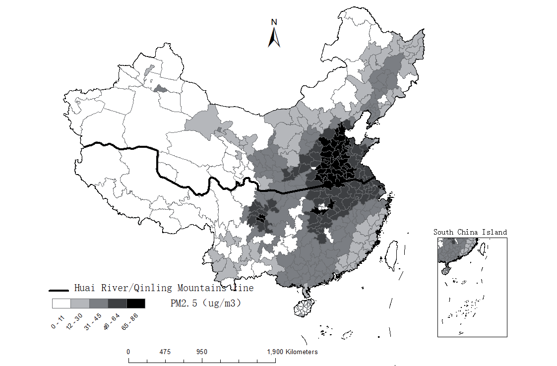
China’s winter heating policy refers to the government’s centralized winter heating for cities north of the Huai River/Qinling Mountains line, China’s north-south border. The government bases central heating on this line for three reasons. First, because the average temperature in January is around zero degrees Celsius, northern cities have a greater requirement for heating. Second, because this line is not used for other administrative purposes, it can help to reduce policy discrimination [24, 25]. Third, the government only provides central heating for northern cities, reducing energy consumption and financial expenditure [26, 27]. Every winter since 1958, cities north of the border have received government-funded central heating. In contrast, the state provides no central heating in southern China. Coal is used in most northern centralized heating systems. Particulate matter and other air pollutants are released when coal is burned incompletely to generate heat. Pollution from coal heating is primarily local because most of the heat comes from boilers in residential buildings. Therefore, residents in southern and northern China experience significantly different annual exposures to outdoor air pollution due to heating in the winter. Multiple studies have found that China’s central heating policy has resulted in significantly higher outdoor average total suspended particulate matter levels and PM2.5 concentrations in the north than in the south [26, 28, 29]. Fig. 1. shows the Huai River/Qinling Mountains line of China’s winter heating policy and the PM2.5 concentration in prefecture-level cities along the line in 2010. Intuitively, there are obvious differences in PM2.5 concentrations between the north and south of the Huai River line.
In this study, we use the exogenous changes in air pollution caused by China’s winter heating policy to estimate the impact of outdoor exposure to air pollution on adult body weight.
Econometric Model and Data
Empirical Strategy
The goal of our empirical estimation is to capture the causal effect of long-term air pollution on adult body weight. There are two important challenges to doing this. The first one is omitted-variable bias. Air pollution and economic activity are highly correlated. Urban residents with high economic activity have higher incomes. It has been documented that exogenous family income subsidies can significantly increase the weight level of children and increase the risk of overweight and obesity [14]. Thus, it is likely the case that those cities with high-paid jobs and per capita income are also those that experience high levels of air pollution. In fact, as the confounding factors related to economic activities cannot be fully observed, air pollution and body weight may show a correlation over time. Ignoring the regression results of confounding factors should not be interpreted as the impact of air pollution on body weight, because time-varying confounding factors such as economic activity could be driving the correlation. Second, despite the fact that air pollution is not likely to have an effect on body weight directly, it may have an indirect effect on body weight through several behavioral pathways, which means that overweight and obesity may be the result of the long-run accumulation of air pollution. However, some literature has only provided short-run changes in air pollution and body weight [10, 21]. Therefore, we expect that overweight and obesity outcomes in individuals should be a response to behavioral habits shaped by observable long-run changes in air pollution. The interaction of these two challenges creates a considerable identification challenge since it is challenging to identify sources of long-run fluctuation in air pollution that are unrelated to other sociodemographic or economic trends. Our strategy for overcoming this challenge is to build a 10-year annual average exogenous variation at the county level between 2001 and 2010 in pollution caused by the winter heating policy, which offers coal-fired centralized indoor heating to the north of the Huai River/Qinling Mountains line but none to the south. Specifically, we use an RD design implicit in the winter heating policy to measure its impact on air pollution and adult body weight2. We examine separately whether the winter heating policy led to discontinuous changes in air pollution and adult body weight north of the river line. Any unobserved drivers of air pollution or adult body weight must change smoothly as they cross the river, which is the respective required assumption. Local linear regressions on either side of the river, or adjustment for a sufficiently flexible polynomial in distance from the river line, can eliminate all potential omitted-variable bias and enable causal inference if the relevant assumption is true.
The recent literature suggests that a local linear regression based on data near the RD cutoff is likely to produce the most robust estimates [31, 32], and the parametric RD approach is found to have several undesirable statistical properties [32]. Therefore, we use local linear regression as the main specification and emphasize our results from the non-parametric regression method. We also present outcomes for the RD approach using parametric estimation in robustness checks. In practice, we propose the following setup for estimation by local linear regression:
Where Yic denotes the body mass measures, including BMI, and indicators for overweight and obesity for individual i residing in county c. Pic refers to the average outdoor exposure annual average concentration of PM2.5 sustained by individual i residing in county c. Note that overweight and obesity may be the result of long-term exposure air pollution, and in this study, we specified a 10-year period for exposure to air pollution to affect body weight. Nic is the dummy variable for the north, dic, the running variable, is the distance between individual i residing in county c and the Huai River border. εic and uic are the error term. Temperature, relative humidity, cumulative precipitation, and sunshine duration are all covariates Xic. Zic is a vector of observed factors that may have an impact on health, which includes not just Xic, but also demographic and health behavior characteristics.
To solve the attenuation bias associated with the mismeasurement of air pollution, we estimate the effect of PM2.5 on adult body weight using a fuzzy RD framework with a second-stage regression3 specified by equation (3):
by using Nic as the instrument for Pic. The identification presumption is that there is no correlation between the instrument and the error term σic. The parameter of interest is φ1, which measures the effect of PM2.5 exposure on BMI, overweight, and obesity of adults after controlling for available controls. The other variables are as described above.
Data
We calculate BMI as an individual’s weight in kilograms divided by the square of their height in meters (kg/m2). We determined overweight and obesity in adults based on the Chinese reference4, which defines an adult as overweight if their BMI is greater than or equal to 24, and obese if their BMI is greater than or equal to 28. Since a child’s weight status is determined using age- and sex-specific percentiles for BMI, referred to as BMI-for-age, rather than the BMI threshold used for adults, our sample exclusively comprises adults (those above the age of 18).
Given that the dependent variables in this paper were calculated from both weight and height, we obtained individual self-reported height and weight data from the China Family Panel Studies (CFPS), a large-scale national social tracking survey. CFPS tracks and collects data at the individual, family, and community levels to reflect changes in China’s society, economy, population, education, and health. The CFPS 2010 wave, which serves as a baseline survey and interviews 14960 households and 42590 persons from 162 counties/ districts in 25 provinces, covers 95% of the population in China. Using implicit stratification, multi-stage (county/district, village/community, and household), multi-level, probability sampling in proportion to population size, the Social Science Research Institute at Peking University conducts the CFPS. Our data on the key independent variable, i.e., the running variable, is obtained in two steps. We initially utilized ArcGIS to extract the longitude and latitude of the 162 counties surveyed from the CFPS map of China. We then use ArcGIS specifically to calculate the shortest distance between the county centroids and the closest location along the Huai River border.
We use PM2.5 to measure air pollution because Wang et al. (2014) [33] showed that high ambient PM2.5 concentrations are thought to be closely related to China’s enormous primary energy consumption, especially coal consumption. Our PM2.5 data comes from satellite-based Aerosol Optical Depth (AOD) retrievals to reduce subjectivity errors. Consistent with other literature [34], we obtain the AOD data from the Atmospheric Composition Analysis Group of Dalhousie University through the sensor and process it with ArcGIS software. To estimate the effects of long-run air pollution exposure, we aggregate from grid to county for each year and further average the 10-year exposure window between 2001 and 2010.
Weather controls are among our covariates. We obtained weather data from the China Meteorological Science Data Sharing Service Website’s Daily Data Set of China’s Surface Climate Data, which publishes daily weather variables from over 800 meteorological stations in China. To convert weather data from stations to counties, we use the inverse distance weighting method and a radius of 200 km. Temperature, relative humidity, total precipitation, and sunshine duration are all included in the weather data. This dataset has been used in previous studies [35, 36]. We calculated the annual average of the weather data from 2001 to 2010 to match the air pollution data. Other covariates such as age, gender, minority, urban/rural status, income, and health behavior variables such as whether the respondent smokes and drinks regularly are obtained from the wave of 2010 in CFPS.
We matched the average processed pollution data and weather data to the wave of 2010 in the CFPS baseline survey to meet the requirements of the Huai River RD design for cross-sectional characteristics. Our final sample has 32511 adult individuals from 162 counties/ districts across 25 provinces.
Results
Descriptive Statistics and Transparent Graphics of RD Design
Table 1. reports summary statistics for key variables. We aim to estimate the effect of air pollution on body weight. We use three indicators to measure body weight: BMI and the indicators for overweight and obesity. We divided the sample into two groups south and north of the Huai River line for summary statistics. In our sample, the mean BMI in the north was 22.59 in 2010, with a standard deviation of 3.44, while in the south it was 21.88, with a standard deviation of 3.25, both close to the cutoff of 24 for overweight. Correspondingly, the mean overweight and obesity rates in the north were 31% and 7%, respectively, compared to 24% and 4% in the south. Since BMI is calculated from body height and weight, we also report the average height and weight. The average weight in the north was 61.63 kg, and the average height was 1.65 m. The average weight in the south was 57.83 kg, and the average height was 1.62 m. In terms of body height, the south and the north are very close, which provides us with the opportunity to exclude some confounding factors since our sample only includes adults whose height does not respond to pollution exposure and also suggests that the difference in BMI between the south and the north is mainly dominated by body weight.
We used PM2.5 concentrations to measure air pollution. The average PM2.5 concentration was 49.41 in the north and 43.85 in the south, both of which exceeded the cutoffs given by the WHO for concentrations that could be potentially hazardous to health.
Table 2. reports summary statistics for control variables. Weather controls are at the county level, with demographic and health behavior characteristics serving as individual-level controls. We construct individual-level control variables from CFPS. Survey respondents were asked to self-report their age, gender, minority, urban/rural status, income, and whether they smoked and drank regularly. These control variables are useful for two reasons. First, individual-level controls are important confounders in estimating the long-run health effects of air pollution. Second, weather controls can affect both air pollution and body weight. In addition to dividing the sample into two groups south and north of the Huai River line for summary statistics, Table 2. extends Table 1. by comparing the differences between the two groups. Column (3) reports the mean differences between north and south and the associated standard errors. It is worth noting that the statistic shows a simple difference, not necessarily a discontinuous difference at the border.
These control variables are observable determinants. The RD design’s identifying assumption is that observable determinants change smoothly at the boundary. Column (4) shows RD estimates for weather and individual-level observable covariates. Each RD estimate uses local linear regression. Each variable’s optimal bandwidth is chosen separately using two different mean square error (MSE) optimal bandwidth selectors proposed by Calonico et al. (2014) [37], Calonico et al. (2018) [38], and Calonico et al. (2019) [39] with a triangle kernel. We cannot detect major changes in these variables, suggesting that observable determinants change smoothly at the boundary.
Table 1.
Summary statistics of key variables.
[i] Note: The CFPS baseline survey sampled 83 northern and 79 southern counties in China. The pollution variable is at the county level, and the body weight variable is at the individual level. Each individual’s BMI measurement uses their weight in kilograms divided by the square of their height in meters (kg/m2). Overweight is a dummy variable equaling 1 if the BMI is greater than 24. Obesity is a dummy variable equal to 1 if the BMI is greater than 28.
Table 2.
Summary statistics of control variables.
[i] Note: Columns (1) and (2) report the mean values of the boundary’s north-south samples, while Column (3) reports the raw differences between the means of the two samples using the t-test. The nonparametric RD estimation results are shown in Column (4). Standard deviations are reported in parentheses in Columns (1) and (2). Standard errors are reported in brackets in Columns (3) and (4). * significant at the 10% level; ** significant at the 5% level; *** significant at the 1% level.
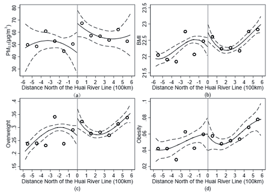
The RD method allows for a transparent graphical representation of the effect of interest. Before discussing the estimation results, we visualize the patterns of air pollution and body weight in the data. We separately plotted the variation of PM2.5, BMI, overweight, and obesity rates across the Huai River line in Fig. 2. The X-axis indicates the north-south distance from the county to the Huai River line. We plot the quadratic polynomial fit, along with the 95% confidence interval, against distances around the boundary. It is apparent that there is a discontinuity of PM2.5 concentration, BMI, and overweight rate increases at the boundary, suggesting that the winter heating policy has caused higher pollution levels, average BMI, and overweight risk in the northern counties of the Huai River boundary.
Main Results
Table 3. presents the estimated discontinuities of the PM2.5 average concentrations and body weight across the boundary by running equations (1)-(3). All estimations use the triangle kernel and report the conventional RD estimates with traditional standard errors. Panel A presents the first-stage estimation results for PM2.5. Panels B and C report the results of reduced form and fuzzy RD estimation, where the dependent variable is body weight measure, respectively. In Column (1), we do not add any controls, and weather controls are included in Column (2). In Column (3), we further add detailed individual-level demographic and health behavior characteristics. There are no observable confounders at the individual level in Panel A since they are significant confounding factors that may affect health rather than air pollution5. The optimal bandwidth uses two different MSE-optimal bandwidth selectors proposed by Calonico et al. (2014) [37], Calonico et al. (2018) [38], and Calonico et al. (2019) [39]. We prefer the estimates from the most comprehensive specification (Column (2) for Panel A, Column (3) for Panels B and C).
Fig. 2.
Distribution of pollution exposure and body weight at the Huai River line. Note: The graphs show the average value north and south of the Huai River line. The horizontal axis is the distance north (positive values) and south (negative values) from the sample location to the Huai River line. The scatterplot is the means within 100 km bins, and the solid and dashed lines are the regression fit and associated 95% confidence intervals, respectively.
In Panel A, we find a strong first-stage relationship. The estimated coefficients are stable across the specifications and statistically significant at the 5% level. Column (2), our preferred specification, suggests that the winter heating policy has increased PM2.5 concentrations in the past 10 years by 20 μg/m3; this translates into a 45% increase at the Huai River boundary (the mean PM2.5 concentrations in the same period south of the Huai River border are 44 μg/m3).
Panel B estimates the impact of the winter heating policy on body weight measurement and finds that the winter heating policy increases BMI by 0.315 units and the probability of being overweight by 6%. There is a statistically significant discontinuous increase in the risk of being overweight at the boundary, but not in the risk of being obese. Adults living north of the Huai River line have a substantially higher risk of being overweight than those living south. These results echo the graphical analyses that the winter heating policy can cause a significant deterioration in the air quality in northern Chinese cities and increase the risk of being overweight.
Given that many counties have good air quality because of environmental regulations, despite being located north of the Huai River border. Therefore, the reduced form estimate (Panel B) overvalues the effect of the winter heating policy. Panel C reports the fuzzy RD estimates of the impact of air pollution on various indicators of body weight. We prefer the result in Column (3), where both weather conditions and demographic and health behavior covariates are controlled. Column (3) of Panel C shows that a 1 μg/m3 increase in average PM2.5 concentrations in the past 10 years has increased BMI by 0.014 units and the probability of being overweight by 0.3 percentage points. We find a statistically significant effect of PM2.5 on the risk of being overweight, but not on the risk of being obese. These findings are remarkably stable and are not affected by the inclusion of different controls.
Two features are noteworthy when comparing the results of Deschenes et al. (2020) [11], who studied the effect of air pollution on body weight using thermal inversion as an instrumental variable for air pollution. First, we found that the results of air pollution on BMI and overweight rates were similar in sign and magnitude to those of Deschenes et al. (2020) [11]. Second, we did not find a statistically significant effect of air pollution on the probability of adult obesity, but the results estimated by Deschenes et al. (2020) [11]. were statistically significant. The important reason is that Deschenes et al. (2020) [11]. estimate a global effect, while our RD design estimates a local effect. In our local estimates, many geographic samples will be excluded, and overweight and obesity are likely to have significant geographic characteristics. Despite the differences, we fail to observe contradictions with the main findings of Deschenes et al. (2020) [11].
Table 3.
RD and OLS estimation results.
[i] Note: Columns (1)-(3) are the nonparametric estimated discontinuity at the Huai River obtained using local linear regression and two different MSE-optimal bandwidth selectors with a triangle kernel. Each RD estimate reports conventional results and has an asymmetric optimal bandwidth on both sides of the threshold. Column (4) presents the OLS regression, in which running variables are not included in the regression equation. Weather controls include temperature, relative humidity, precipitation, and sunshine duration. Individual controls include age, gender, minority, urban/rural status, income, smoking regularly, and drinking regularly. Standard errors are reported in parentheses. * significant at the 10% level; ** significant at the 5% level; *** significant at the 1% level.
For comparison, Column (4) also presents the traditional OLS estimates that do not include a running variable. We discover that the magnitude of the RD estimates is smaller than the OLS estimates. There are two possibilities for such a difference. First, OLS results are biased upward possibly, due to omitted variable bias. The second explanation is an outdoor air pollution exposure measurement error. We do not know the specific exposure of each individual because we are using area-level outdoor air pollution. Many studies on the effects of air pollution in the literature have noted that assigning air pollution exposure to individuals from the area level (in our study, the county level) introduces classical measurement error [40-43]. The possible reasons that outdoor air pollution exposure increases the risk of obesity are as follows: First, air pollution affects people’s dietary behavior. For example, air pollution may trigger depression and anxiety, which increase the appetite for food and lead to excessive food intake. Second, air pollution affects people’s exercise behavior. Air pollution causes people to stay indoors and reduce the amount of outdoor exercise. Changes in diet and exercise behavior increase the risk of obesity by creating an energy imbalance between calories consumed and calories expended.
Robustness Checks
In this section, we examine the qualitative effects of the choices we made in our study along a variety of dimensions on our primary findings.
We first experiment with a parametric method to examine the sensitivity of our results. Since the consistency of parametric estimation requires controlling a flexible polynomial, we also check the robustness of our parametric results for higher-order polynomials. The implementation of local linear regression for parametric estimation requires manual bandwidth limitations. We refer to Ebenstein et al. (2017) [28] to manually limit the bandwidth within 500 kilometers from the north to the south of the Huai River line. Table 4. has the results using the parametric method when the order of the polynomial varies between linear and sextic. Panels A and B present the reduced form and fuzzy RD parametric estimation results, respectively. The RD-estimated effects on BMI and overweight are always significantly positive. Our results are robust to the choice of functional forms for the RD polynomial. Overall, our parametric and nonparametric estimates are qualitatively similar to those in our primary analysis and suggest that our major findings in this study do not depend on parametric or nonparametric estimation methods.
Second, we probe the sensitivity of the results to different bandwidth selection and kernel weighting methods. Table 5. shows the non-parametric results. All regressions use an asymmetric bandwidth. We replicated Column (3) of Table 3., our preferred specification, as the baseline regression results and placed them in Column (1). In our preferred specification, we use triangle kernel local linear regressions and the bandwidth selected by the MSE-optimal bandwidth selector. To check the robustness of the results to different kernel functions, we report the estimation results to different kernel types (Epanechnikov and Uniform) in Columns (2) and (3). To verify the sensitivity of our results to different bandwidths, in Columns (4)- (6), we replace the optimal bandwidth selection method and execute the kernel weighting method in a sequence consistent with Columns (1)-(3). We estimate the effect of winter heating policies on body weight using the coverage error rate (CER) optimal bandwidth method proposed by Calonico et al. (2018) [38], Calonico et al. (2020) [44], and Calonico et al. (2022) [45]. In general, we find that the results are similar in sign and magnitude to those in Table 3., suggesting that our results are robust to these alternative bandwidth selection and kernel weighting methods.
Table 4.
Robustness test for parametric estimates.
[i] Note: This table shows the parametric RD estimation results of polynomials of different orders. The optimal bandwidth is manually limited to 500 kilometers from the north to the south of the Huai River line. All regressions include weather and individual controls. Standard errors are reported in parentheses. * significant at the 10% level; ** significant at the 5% level; *** significant at the 1% level.
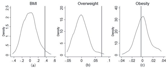
Third, to exclude the possibility that our estimates are likely to be systematic artifacts caused by spurious factors around the Huai River line, we implement a set of repeated placebo exercises with randomly varying latitudinal boundaries in the sample. Each placebo estimate computes a “false” running variable as the distance from the sample location to the placebo boundary and estimates the discontinuity in the body weight at the placebo boundary. We use a triangle kernel local linear regression and the bandwidth selected by two different MSE-optimal bandwidth selectors to estimate the effect of the boundary on body weight. Fig. 3. compares such estimates with a distribution of 500 placebos. The distributions of the placebos are centered at 0, and the probability of obtaining values below the estimates at the true boundary for BMI and overweight is both less than 0.05. Under the null hypothesis of no effect of China’s winter heating policy, the estimating bias is sufficiently large to account for the magnitude of the estimated coefficient. These results seem to rule out the possibility that our main results are systematic artifacts caused by spurious factors around the Huai River boundary.
Finally, we also explore various robustness checks for alternative specifications, variables, and overweight and obesity reference standards in Table 6. For nonparametric RD estimates in Table 6., we use the triangle kernel local linear regressions and the bandwidth selected by two different MSE-optimal bandwidth selectors as the preferred specification. We first examine the robustness of our results to the WHO reference standard, which defines the BMI threshold of adult overweight as 25 and obesity as 30. Column (1) presents the RD estimates using the alternative standard. Although the coefficient was different in magnitude, the effect on body weight from this exercise is similar to the main results presented in Table 3. Thus, our results are robust to this alternative reference. BMI is calculated from body weight and body height. We estimated the results for body weight and height as dependent variables separately. We expect that the effect on height should be insignificant because our sample includes only adults, whose height should not respond to air pollution. Columns (2) and (3) present the results of the estimation of weight and height, respectively. As expected, we find a statistically significant effect on weight and height, but the coefficient of height is very small, suggesting that the effects of winter heating policies on BMI are mainly mediated through body weight.
Table 5.
Robustness test for alternative bandwidth selection and kernel weighting methods.
[i] Note: Each RD estimate uses local linear regression and asymmetric bandwidth. Each cell in the table represents a separate RD estimate and has the optimal bandwidth for both sides of the threshold. All regressions include weather and individual controls. Standard errors are reported in parentheses. * significant at the 10% level; ** significant at the 5% level; *** significant at the 1% level.
Fig. 3.
RD estimates of the effect of the latitude boundary on body weight, placebo estimates. Note: The graphs show the distribution of the RD estimates obtained by using a nonparametric method obtained from 500 random permutations of the boundary. The vertical red solid lines denote the actual estimates.
Migration will confound our study in two ways. On the one hand, there may be migration from a county of hukou registration (obtained at one’s county of birth) to another county to work or to seek cleaner air. If such migration occurs, our pollution exposure measurements may be subject to error because we assume that pollution exposure levels are those observed in their county of hukou registration. On the other hand, migration may be cross-border, which would pose a potential challenge to our RD design if such migration were to be substantial. Several studies have shown that actual cross-border migration rates are low due to strict immigration policies [24, 28]. Therefore, migration may not have a significant impact on our estimated results. We consider two approaches to exploring the potential impact of migration on the results. First, to address the challenge of RD identification due to cross-border migration, we exclude samples without local hukou registration. Second, job-oriented migration usually occurs within prefecture-level cities; thus, we collapse the pollution data for prefecture-level cities for RD estimation. The results are presented in Columns (4) and (5), respectively, and fail to contradict the study’s qualitative findings. Pregnant women may influence our estimates. Their body weight increases significantly during pregnancy, so their BMI cannot be defined as overweight or obese by conventional standards. Since there are no questions about pregnancy in the questionnaire, we further restrict the age of the sample to women over 50 years old. Column (6) of Table 6. reports similar findings.
Mechanism Tests
The underlying cause of overweight and obesity is an energy imbalance between calories consumed and calories burned, which is mainly caused by excessive food intake and a lack of physical activity. Thus, we explore two possible channels through which PM2.5 could affect body weight. First, air pollution leads to higher food intake. The mechanism through which this occurs is the following: Air pollution is likely to induce depression and anxiety, and anxiety may release the hormone cortisol [46], which increases the appetite for food, leading to excessive food intake. For concreteness, we explore differences in food intake to explain air pollution’s effects on body weight. Given that residents north of the Huai River boundary have higher levels of exposure to pollution, they may have a higher average food intake than residents south of the river boundary. Specifically, we examined differences in adult red meat intake, which is closely related to body weight, across the Huai River boundary.
Second, air pollution may also affect weight by reducing physical activity. For example, when faced with outdoor air pollution, people may choose to stay indoors to avoid it, resulting in an increase in physical inactivity due to indoor sedentariness. These behaviors can lead to an energy imbalance between calories consumed and calories expended, which increases the risk of fat accumulation and obesity. Exercise lowers the risk of obesity, according to prior research [47-49]. We investigate differences in physical activity among people on each side of the Huai River line under the hypothesis that variations in physical activity are related to outdoor pollution. We examined information on individuals’ dietary patterns and exercise habits as documented in the CFPS data to get insight into these issues. Under our main specification, we explored the impact of China’s winter heating policy on the exercise and food intake of adults.
Table 6.
Robustness test for alternative specifications and variables.
[i] Note: Each cell in the table represents a separate RD estimate. Each RD estimate uses local linear regression and triangle kernel weights. Column (1) reports the estimates using a WHO standard for adults overweight and obese, which defines the BMI threshold of adults overweight as 25 and obesity as 30. Columns (2) and (3) report the results of RD estimation for weight and height as dependent variables, respectively. Column (4) excludes samples without local hukou registration. Column (5) collapses pollution data at the prefecture level, which typically includes 5 to 15 counties. All regressions include weather and individual controls. Standard errors are reported in parentheses. *significant at the 10% level; ** significant at the 5% level; *** significant at the 1% level.
Table 7. presents the reduced form and fuzzy RD of the winter heating policy on the dietary intake and physical exercise of adults. All estimates use two different MSE-optimal bandwidth selectors proposed by Calonico et al. (2014) [37], Calonico et al. (2018) [38], and Calonico et al. (2019) [39]. Columns (1) and (2) report the reduced form and fuzzy RD results, respectively. We start with food intake in Panel A. As mentioned earlier, we expect air pollution exposure to increase meat intake and decrease vegetable intake. We find that the winter heating policy had a positive effect on meat intake and a negative effect on vegetable intake, indicating that food intake is a possible channel for air pollution effects. We then examine the effect of the winter heating policy on physical exercise. We constructed a physical activity frequency variable using CFPS. Respondents were surveyed on their self-reported frequency of fitness or physical activity participation, ranging from 1 (almost daily) to 5 (1 time in a few months). We find that outdoor air pollution exposure reduces the frequency of physical activity in adults, suggesting that reduced outdoor physical activity to avoid air pollution is a possible channel for air pollution effects.
Discussion
Being overweight and obese can induce a variety of chronic diseases, including hypertension, diabetes, coronary heart disease, and stroke, and thus contribute significantly to social medical costs. To clarify the economic costs of being overweight caused by air pollution, we perform a calculation that multiplies the health expenditures caused by being overweight using an estimated coefficient of interest, φ1, which measures that the prevalence of overweight increases by φ1 for every 1 μg/m3 increase in PM2.5 concentration. Because it is often challenging to calculate accurate and up-to-date data on health expenditures attributable to overweight, we want to emphasize that our calculation below should be interpreted as a back-of-the-envelope calculation.
Table 7.
Potential mechanisms of the winter heating policy on body weight.
[i] Note: Each cell in the table represents a separate RD estimate. Each RD estimate uses local linear regression and triangle kernel weights. The dependent variable “Meats/ Fishes” is a dummy equal to 1 for an adult who consumed meat/fish more than 10 times a week on average in the past three months and 0 otherwise. Vegetables and puffed/fried foods in Panel A are the average weekly consumption times of an adult in the last three months. The dependent variable in Panel B is the frequency of an adult’s fitness or physical exercise, ranging from 1 (almost daily) to 5 (1 time in a few months). All regressions include weather and individual controls. Standard errors are reported in parentheses.
Using data from the 2002 wave of the China Health and Nutrition Survey and the Third National Health Service Survey in 2003, Zhao et al. (2008) [50] calculated that the direct economic burden of hypertension, diabetes, coronary heart disease, and stroke due to overweight/obesity in China in 2003 was 21.11 billion CNY, accounting for 3.2% and 3.7% of the total health and medical costs in China. Therefore, the minimum health expenditure related to overweight/ obesity is 21.11 billion CNY. Since we find that a 1 μg/m3 increase in average PM2.5 concentrations increases the prevalence of overweight by 0.3 percentage points (Panel C of Table 3.), we can conclude that a reduction of 1 μg/m3 of PM2.5 concentration will bring 63.33 million CNY of health benefits by reducing the medical costs related to overweight.
China has been heavily dependent on coal for power generation, and in response to air pollution caused by coal burning, the Chinese government has in recent years launched a program to replace some coal-fired power plants with cleaner energy sources such as natural gas or wind power. The replacement of coal power plant policies was first piloted in Beijing starting in 2014 and later expanded to several provinces in northern China. In the winter of 2017, Beijing and several surrounding cities banned coal heating altogether and were required to switch to natural gas. The policy has proven to have an immediate impact on reducing air pollution. For example, Beijing’s average PM2.5 concentration was reduced by 50% in December 2017 compared to air pollution levels in 2014.
To shed light on the range and magnitude of the costs and benefits of the energy replacement policy, we first check the emission inventory from China’s coal power plants. Ma et al. (2017) [51] imply that 15.5% of North China’s PM2.5 emissions come from coal burning in power plants during the winter. Assuming that a 15.6% decrease in PM2.5 corresponds to an average PM2.5 concentration decrease of 15.6%, this results in a 7.7 μg/m3 decrease in PM2.5 concentration for the average nationwide level of PM2.5 concentration in our data. The application of the study’s estimates suggests that the replacement policy will generate 488.04 million CNY of benefits because it will save medical costs that are overweight-related.
For the cost of replacing coal with natural gas, we need to assume some key elements of cost since the Chinese government did not provide an estimate of the total cost of the policy. The cost of a coal-to-gas policy should include at least three elements: first, infrastructure costs, such as pipeline construction and gas stove expenditures, second, higher fuel costs, and third, the lifetime of the infrastructure. Fan et al. (2020) [25] calculate the total cost of replacing coal with natural gas for a planned 20-year operation to be between CNY 1016 billion and CNY 1108 billion per year.
Comparing the cost estimates to the benefit estimates, we see that the costs of replacing coal with natural gas outweigh the benefits. However, note that the cost estimate led by Fan et al. (2020) [25] is based on the total cost of the coal-to-gas policy, while our benefit estimate only focuses on the impact of air pollution on overweight. If we include other health benefits of air quality improvements, including lower premature deaths, reduced defensive expenditures, and life expectancy maintenance, the health benefits of the coal-to-gas policy would greatly exceed the costs. In conclusion, although the benefits associated with reduced overweight represent a small percentage of the total health benefits of air quality improvements, we should not ignore the positive effects of air quality improvements on overweight. This is because we are likely to underestimate the benefits associated with being overweight for two reasons. First, being overweight not only increases the risk of many chronic diseases but also affects labor productivity. Second, the overweight and obesity epidemic is growing rapidly. WHO reports that the global prevalence of overweight and obesity almost tripled between 1975 and 2016 [2], which exceeds the rate of GDP growth during this period, and health expenditures typically increase with GDP growth, making our estimates low-bound.
Conclusions
This paper sheds light on how increased air pollution exposure affects adult body weight in the long term. We focus on the winter heating policy in China to address the endogeneity problem. Specifically, we used a geographic RD framework to estimate whether there were discontinuous changes in BMI, overweight, and obesity depending on whether they were located north or south of the Huai River line.
We find that the average BMI and rates of overweight are about 0.315 units and 6.1 percentage points higher in the north, owing to higher outdoor air pollution exposure. More generally, a 1 μg/m3 increase in PM2.5 concentration increases the BMI by 0.014 units and the probability of being overweight by 0.3 percentage points. The effect of air pollution on being overweight is robust across various specifications. The rising risk of being overweight caused by air pollution is mainly through channels such as increased intake of energy-dense foods and less physical exercise.
Finally, we conduct a cost-benefit analysis to evaluate the economic benefits of the coal-to-gas policy. We mainly consider the savings in medical costs associated with overweight reduction as benefits. We find that the costs of replacing coal with natural gas and electricity outweigh the benefits. However, we believe the benefits of the coal-to-gas policy will greatly exceed the costs if we include other sources of indirect benefits, such as lowering premature deaths and gains from improved labor productivity. There are still open questions for future research, including the effect of coal-to-gas policy on body weight.
This study contributes to a broad discussion of the relationship between air pollution and health costs. Our results indicate that the current emphasis on common NCDs such as cardiovascular diseases and diabetes-related costs understates other hidden costs of pollution on being overweight. If we count these additional costs, the benefits of reducing pollution would be higher. From a policy perspective, evaluating the impact of air pollution provides useful information for environmental policies. When considering such things as replacing coal with natural gas or an air quality improvement program, social planners should not ignore its positive effect on reducing the risk of being overweight.