

Introduction
Global warming is a threat to the survival of mankind [1]. As the world’s largest carbon emitter, China has been committed that it would achieve carbon peaking by 2030 and carbon neutrality by 2060. Agricultural carbon emissions (ACEs) are the second-largest source of global carbon emissions [2]. China’s ACEs account for 17% of the country’s total carbon emissions, but the number is 13.5% in the world at large. Hence, China’s agriculture sector has huge potential to reduce its carbon emissions [3]. Most ACEs come from pesticides, fertilizers and other inputs and energy consumption in agricultural production, which are necessary for production activities, but they also cause climate warming and threaten ecological security [4, 5]. As the mainstay of agricultural production, rural labor plays a crucial role in the allocation of agricultural resources and the use of agricultural land, which has an important impact on ACEs.
At present, China is in a stage of rapid development of a new type of urbanization, with a large number of laborers emigrating from the countryside to the city. China’s outline of the vision goal for 2035 clearly emphasizes that it will deepen the reform of the household registration system so that the urbanization rate of China will reach about 72% in 2035. Urbanization leads to changes in traditional agricultural production modes and land use, thus affecting ACEs [7, 8]. Therefore, this paper selects China as the research object to explore the effect of urbanization on ACEs, including internal mechanisms, spatial spillover effects, and regional heterogeneity. The main innovation is to incorporate China's agricultural land production mode into the theoretical mechanism framework of urbanization and ACEs and test it empirically. It can provide theoretical value and data support for future related research and application value for the scientific formulation of ACE reduction policies in China and other countries.
The remainder of this paper is organized as follows: Section 2 summarizes the literature; Section 3 consists of the theoretical analysis and research hypotheses. After that, Section 4 introduces the material and methods; Section 5 presents results and discussion; and Section 6 elaborates the conclusion of this paper.
Literature Review
The research on ACEs is mainly divided into two categories. One category is the calculating method of ACEs, and the other is the analysis of its influencing factors. In terms of ACEs calculations, there are no recognized methods. Early scholars only measured the ACEs of the planting industry from the perspective of agricultural materials [10]. Later, the agricultural production methods and agricultural inputs are taken into account to measure ACEs [3], and the types of agricultural carbon sources extended from 6 to 16 categories, mainly including farmland use, rice fields, livestock enteric fermentation, and manure management [11, 12]. In addition, some scholars also calculate ACEs from both direct and indirect energy consumption perspectives [13, 14]. In general, the calculation of ACEs has gone through a process of increasing accuracy in methodology and gradual expansion of the range of carbon sources. In terms of ACEs’ influencing factors, most of the existing literature was conducted from the perspective of agricultural production factors and production methods, including economic growth, labor, finance, technology, and policy. Generally, the relationship between ACEs and agricultural economic growth shows a bidirectional causality in both the short-run and the long-run [15]. It was found that the proportion of the rural population is negatively correlated with ACEs [16], and the decline in the level of rural human capital exacerbates ACEs [17]. Finance, such as rural inclusive finance, digital finance, and green finance, can all affect agricultural activities through some intermediate mechanisms, thus affecting ACEs [18, 19]. Technological progress has a significant impact on ACEs, but the direction of the impact is uncertain, because it includes not only progress in green technologies but also that in non-green technologies [20, 21]. For example, the energy rebound effect of technological progress aimed at improving agricultural labor productivity has a complex impact on ACEs [22, 23].
Most studies focus on the effects of urbanization on industrial carbon emissions and total carbon emissions, but there are few studies on the relationship between urbanization and ACEs [27-29]. Some scholars divided urbanization into different dimensions and studied the heterogeneous effects of them on ACEs, such as population, economy, land, employment, and social urbanization [32, 33]. The spatial spillover effect and spatial heterogeneity of the impact of urbanization on ACEs are also concerns. It was found that both urbanization and ACEs have a significant spatial correlation, and the impact of urbanization on ACEs in the western region is stronger than that in the central and eastern regions [9, 34]. Additionally, urbanization is also taken as a moderating variable to study its moderating effect on the relationship between a certain factor and ACEs in some studies. For example, Chang [35] found that urbanization has a positive moderating effect on digital finance’s ACE reduction effect.
Regarding the impact of agricultural land use change on ACEs, scholars generally analyzed the effects offrom fertilizer and pesticide use, crop cultivation structure, cultivation scale, and agricultural machinery. It is obvious that excessive fertilizer and machinery are important factors affecting ACEs [36]. Liu and Xiao [37] employed the moderated mediating effect model and found that there is a U-shaped relationship between farmland management scale and ACEs. Xu et al. [38] found that agricultural services have a significant role in promoting agricultural green total factor productivity, with ACE as an unexpected output. Rehman et al. [39] found that the reduction of agricultural land affects ACEs in both the short and long term.
In summary, a wealth of research has been done on urbanization and carbon emissions, respectively, providing the necessary theoretical basis, data support, and empirical references for future in-depth studies. However, most studies focus on the relationship between urbanization and industrial carbon emissions, or total carbon emissions, while there are few studies on the relationship between urbanization and ACEs. In addition, the existing studies on the relationship between urbanization and ACEs only empirically test the direct impact, but do not delve into the transmission mechanism and intermediate channel of urbanization affecting ACEs. Therefore, to compensate for the limitations of the relevant studies, with consideration of the reality of China's urbanization process and the specificity of the rural system reforms, this paper further explores the mechanisms underlying the impact of urbanization on ACEs in China.
Different from previous studies, the marginal contributions of this paper are as follows: Firstly, this study constructs an analytical framework including urbanization, agricultural land use change, and ACEs. In addition, the influencing path of urbanization on ACEs is analyzed, including the impact of the scale effect, structure effect, and technology effect. Secondly, this paper constructs a nonlinear intermediary effect model to test the influence mechanism of urbanization and uses the partial differential of the spatial Durbin model to decompose direct effects and indirect effects. In the empirical analysis, the quadratic term of urbanization is introduced to analyze the possible nonlinear impact of urbanization on ACEs. Thirdly, due to regional heterogeneity and spatial correlation, China was divided into north and south, main grain-producing areas, and non-grain-producing areas for heterogeneity analysis according to the regional characteristics of agricultural land. Then, this study investigates the impact of urbanization on ACEs.
Theoretical Analysis and Research Hypothesis
Impact of Urbanization on Agricultural Carbon Emissions
Direct Effect of Urbanization on Agricultural Carbon Emissions
The main manifestation of urbanization is the flow and migration of rural populations to cities. After the large-scale transfer of the rural labor force to the urban non-agricultural sector, the traditional agricultural land utilization mode dominated by labor input has been impacted [40]. China’s early urbanization caused a large amount of resource waste and environmental pollution [41, 42]. In this process, the quantity and quality of the rural labor force declined, so farmers had to use fertilizers, pesticides, machinery, and other factors to replace the labor force. As a result, a large amount of resource waste and ACEs are generated. After China realized this problem, it began to promote agricultural large-scale production and specialized production to improve resource utilization and reduce ACEs. Moreover, with the improvement of urbanization levels, residents have a higher demand for the quality of agricultural products. Therefore, the government guides farmers to develop low-carbon agriculture and organic agriculture, which encourages them to reduce the input of pesticides and fertilizers, and introduce green and low-carbon technologies, thus reducing ACEs [43]. It can be seen that there is not a simple linear relationship between urbanization and ACEs, and urbanization at different stages may have different impacts.
Hypothesis H1: The impact of urbanization on ACEs has phased characteristics, with an overall “inverted U-shaped” relationship in which ACEs show a “first increase, then decrease” as the level of urbanization increases.
Spatial Spillover Effects of Urbanization on Agricultural Carbon Emissions
Urbanization has a spatial spillover effect on ACEs. On the one hand, due to the herd mentality of individual residents, as well as the similarity of transportation infrastructure and economic planning in neighboring areas, the population flow in one area also affects the population flow in neighboring areas, resulting in the mutual influence of regional urbanization level. This is because the change in population will drive a change in demand for agricultural products, which will lead to a change in agricultural resources and energy consumption in surrounding areas and ultimately affect ACEs in those areas. On the other hand, the rural labor flow between provinces promotes the spatial exchange and dissemination of agricultural knowledge, agricultural low-carbon technologies, and specialized production modes, which contributes to the reduction of ACEs [34]. Therefore, the transfer of the rural labor force between different provinces shows the characteristics of spatial dependence and spillover, which deepens the spatial connection between agricultural production and ACEs. Further, this paper proposes the following research hypothesis:
Hypothesis H2: There may be a positive spatial correlation between ACEs and a spatial spillover effect of urbanization on ACEs.
Intermediate Influence Mechanism of Farmland Use Mode
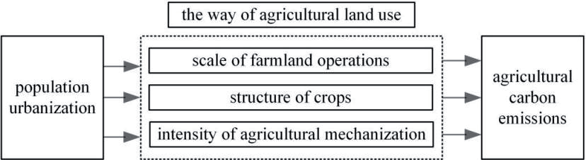
Urbanization affects ACEs through the scale effect, structural effects, and technological effects. The intermediate channel of influence is the way agricultural land is used, including the scale of farmland operations, crop structure, and intensity of agricultural mechanization. The changes in agricultural land use, in turn, affect ACEs. The following is a diagram of the impact mechanisms (Fig. 1).
The impact of urbanization on the scale of farmland has phased characteristics. At the early stage of urbanization, a large number of laborers migrate to cities and towns. The decline in the quantity and quality of rural labor in the process of rural-urban migration leads to a decline in household management ability and restricts the scale of land rented by farmers. Meanwhile, the speed of land transfer lags behind that of population transfer, resulting in inefficient allocation of land resources and a decline in the scale of agricultural land [44]. When urbanization reaches a mature stage, the tide of urbanization drives the gradual improvement of rural land system reform. Because of the agricultural-scale economy effect and specialized production, farmers’ land is concentrated in new operating entities, which promotes the large-scale operation of agricultural land [45]. Further, agricultural land-scale management affects ACEs. Specialized agricultural production and industrial agglomeration generated by large-scale operations are conducive to improving the efficiency of the use of agricultural materials such as fertilizers, pesticides, agricultural film, and agricultural diesel oil. Experienced farmers and professional cooperatives tend to select and apply a more scientific ratio of pesticides and fertilizers and carry out professional soil nutrient management and cultivation protection to reduce the loss of organic carbon during the cultivation process [22].
Urbanization has an impact on agricultural planting structures. On the one hand, the price of grain was relatively low compared with the price of non-grain cash crops, and in view of the increasing cost of rural labor, farmers who calculate “economic accounts” are more inclined to plant cash crops, resulting in the “non-grain” of arable land. On the other hand, in the process of urbanization, the specialized production methods of new agricultural operators tend to be mature, providing favorable conditions for the cultivation of crops with higher specialization and being conducive to reducing the costs of grain cultivation and increasing the proportion [46]. The increase in the proportion of grain cultivation is positive for reducing ACEs. The agricultural inputs such as fertilizers, pesticides, agricultural films, and mechanical energy consumption for the growth cycle of grain are less than those of non-grain cash crops [47]. Existing studies suggest that the rate of soil erosion caused by grain crops is lower than that of cash crops, and the loss of soil organic carbon caused by grain planting is also smaller [48]. Therefore, an increase in the proportion of grain cultivation has a dampening effect on ACEs.
Urbanization is usually accompanied by the optimal allocation of resources such as human, capital, and material resources. The rapid development of the agricultural production equipment or materials sector during urbanization promotes the division of labor based on specialization. The agglomeration and allocation of advanced production factors such as talents, equipment, and technology to agriculture or rural areas promotes technological progress in agriculture [49]. Agricultural technological progress is the “double-edged sword” of ACEs. It includes not only low-carbon technologies with the goal of energy conservation and emission reduction, but also technologies that aim at increasing agricultural productivity, such as high-concentration fertilizer, heavy agricultural machinery, and large-scale irrigation equipment. Moreover, the energy rebound effect of technological advances cannot be ignored [22]. Therefore, the current agricultural technological progress has a dual effect of uncertainty on ACEs. Consequently, this paper puts forward research hypotheses.
Hypothesis H3. Urbanization influences ACEs through scale, structure, and technology effects, which are manifested in three intermediate channels: the scale of farmland operations, crop structure, and agricultural technology progress.
Material and Methods
Model Construction
Baseline Regression Model
Based on the theoretical perspectives of urbanization and ACEs [50]. Drawing on the STIRPAT theoretical model [51], the following baseline model was constructed to examine the impact of urbanization on ACEs for hypothesis H1:
where subscript i is province and t is year; lnnyco2it refers to the logarithm of total ACEs for province i in year t, urbanit denotes the core explanatory variable urbanization rate, urban2it denotes the squared term of the core explanatory variable urbanization rate, and Xit denotes the set of control variables; e1 is the constant term, c1, c2, and ρ1 are the regression coefficients of the core explanatory variables and control variables; ui is the area fixed effects, υi is the time fixed effects, and εit is random disturbance terms.
Intermediary Effects Model
This article draws on the classic equation of the mediation effect proposed by Wen Zhonglin et al. to construct a mediation effect model of the impact of rural urbanization on ACEs [52].
In Equation (2), Mit represents the mediating variable, α1, α2 represents the coefficient of the core explanatory variable and its quadratic term on the mediating variable, and b in equation (3) represents the regression coefficient of the mediating variable on the explanatory variable.
Spatial Econometric Model
In order to test hypothesis 2, it is necessary to measure the spatial dependence of ACEs in China. In this paper, the global Moran’s I index is used to check the spatial correlation of ACEs in 30 provinces across China, calculated as follows:
Where n denotes the 30 provinces of China; xi denotes the ACEs of region i; x̄ denotes the mean value of ACEs in each province and w is the adjacency weight matrix used for spatial effects analysis. Moran’s I index takes values in the range [-1,1], and when the value is greater than 0, it indicates positive autocorrelation; when the value is less than 0, it indicates negative autocorrelation; when the value is equal to 0, it means that there is no autocorrelation.
According to Moran’s I index and its statistical tests, Chinese ACEs were found to be significantly spatially correlated, thus requiring the introduction of a spatial panel econometric model. In this paper, spatial model estimation is carried out by using neighborhood geographic distance weights [53]. The neighborhood geographic distance weights were calculated as follows:
(5)
In the above equation, i and j are the space section numbers, i,j∈[1,n], and n is the number of spatial sections. In contrast, the Queen adjacency rule defines all spatial samples that share a common boundary and common vertices with a spatial sample as their neighboring units. As a result, spatial samples based on the Queen adjacency rule are often more closely related to their surrounding spatial units.
Using the Wald test and LR test to determine the specific form of the spatial panel model. Wald-spatial-lag values and wald-sptial-error values in the Wald test were 144.73 and 156.56, respectively, both rejecting the original hypothesis at the 1% level of significance, and LR -spatial-lag values and LR-sptial-error values were 131.84 and 155.72, respectively, both rejecting the original hypothesis at the 1% confidence level, suggesting that the SDM model cannot degenerate into the SAR model and SEM model, and therefore the SDM model is used in this paper. In addition, the Hausman test statistic rejected the random effect model at the 1% confidence level, indicating that the fixed effect model should be chosen. Meanwhile, the results of the LR effect test all rejected the original hypothesis at the 1% significance level, meaning that the time-space dual fixed effect model is optimal when choosing the SDM model. Therefore, this paper constructs a spatial benchmark model for the effect of urbanization on ACEs as follows:
(6)
where subscript i is the province, j is the neighboring province and t is the year; λ1 are spatial autoregressive coefficients, indicating the influence of ACEs in neighboring regions on local ACEs; θ1, θ2, ρ1 are regression coefficients of explanatory variables and control variables in the region; θ3, θ4, ρ2 represent the influence of urbanization in neighboring regions and control variables on ACEs in the region; μi are regional fixed effects, υt are time fixed effects, and εit is the random disturbance term; Wij is the spatial weight matrix of order 30×30.
Variable Selection
Explained Variable
Logarithm of total carbon emissions from agriculture (lnnyco2). According to the recommended methodology of the 2006 National Greenhouse Gas Inventory Guidelines of the United Nations Intergovernmental Panel on Climate Change [2], the main sources of carbon in agriculture were defined as fertilizer, pesticides, agricultural diesel, agricultural plastic film, crop sown area and agricultural irrigated area. Referring to Li et al. [3], the corresponding emission factors for each carbon source are 0.8956kg/kg, 4.9341kg/kg, 0.5927kg/kg, 5.18 kg/kg, 312.6 kg/km2 and 20.476 kg/hm2. the carbon emission calculation formula as follows:
In the above equation, nyCO2it is total ACEs, Sikt is the carbon emissions from the kth carbon source in province i at year t, Pikt is the quantity of the kth carbon source in province i at year t, and Qk is the carbon emission factor of the kth carbon source.
Core Explanatory Variables
The rate of urbanization of the population (urban) and its squared term (urban2). The urbanization rate is measured as the proportion of the total population living in an urban area. Considering the phased characteristic of the relationship between urbanization and ACEs, the urbanization rate and its squared term are introduced in each model.
Intermediate Variables
(1) Farmland management scale (fms). Drawing on the research of Liu and Xiao [37], the ratio of cultivated land area to the number of people working in agriculture, forestry, animal husbandry and fishery (ha/per) is used to express it. (2) Structure of crops (pgc). It is expressed by the proportion of the sown area of grain crops in the total sown area of crops (%), which can reflect the basic situation of crop structure in each region. (3) Agricultural mechanization intensity (lnami). Agricultural production technologies mainly include labor-saving technologies based on machinery and land-saving technologies based on biochemical inputs, and as the core explanatory variable in this paper is urbanization, agricultural mechanization intensity is chosen as a measure of agricultural technological progress. Drawing on Deng et al.’s [54] study, the logarithm of the ratio of total agricultural mechanization power to total crop sown area (kw/hm2) was used to express the intensity of agricultural mechanization.
Control Variables
Referring to Xu and Lin's [9] research, factors affecting ACEs may also involve the level of economic development, fiscal policy, regional population, industrial structure, and the standard of living of the population. Therefore, the control variables in this paper include: (1) Level of economic development (pergdp): the ratio of regional gross domestic product to regional total population. (2) Population size (pop): the total population of the region. (3) Financial expenditure for supporting agriculture (fesa): the proportion of financial expenditure on agriculture, forestry and water affairs in total financial expenditure. (4) Secondary industry share (secondindu): The proportion of secondary industry output value in regional GDP. (5) Tertiary industry share (thirdindu): The proportion of the output value of the tertiary industry in the regional GDP. (6) Income gap between urban and rural areas (incomegap): the ratio of per capita disposable income of urban households to rural households. (7) Consumption level of rural residents (consumrur): the ratio of consumption of rural residents to the rural population (yuan/per).
Data Source and Descriptive
The data in this paper are obtained from the China Statistical Yearbook, the China Agricultural Yearbook, the China Rural Statistical Yearbook and the statistical yearbooks of each province in previous years. The data used in this study are at the level of 30 provinces (municipalities) in China (excluding Tibet, Taiwan, Hong Kong, and Macao). Due to the difference in the statistical caliber of the data on financial support for agriculture before 2006, the data spans the period 2007-2019. The descriptive results of each variable are shown in Table 1.
Table 1.
Descriptive statistics results.
Results and Discussion
Benchmark Regression and Discussion
Benchmark Regression Results
Since the Hausman test statistic is 96.07, the null hypothesis of random effect is rejected, and the fixed effect model is more appropriate. Therefore, individual fixed (Model 1 and Model 2), time fixed (Model 3 and Model 4), and two-way fixed effect models (Model 5 and Model 6) are used for estimation, respectively.
As can be seen from the last column of Table 2, the estimated coefficient of urbanization rate is 1.653 and its squared term coefficient is -1.542, both of which pass the significance test. It is suggested that the impact of urbanization on agricultural carbon emissions shows a “rising and then falling” trend. The absolute value of the estimated coefficient of the primary term is greater than that of the squared term, indicating that the increase in agricultural carbon emissions caused by the early stage of urbanization is stronger than the emission reduction effect of the later stage.Therefore, promoting urbanization to cross the “abatement effect inflection point” as early as possible will help to further exploit its abatement effect. It is further calculated that the urbanization rate at the inflection point is 53.6%, suggesting that with the advancement of new urbanization, under the premise that other factors are fixed, ACEs are expected to achieve the carbon peak target when the urbanization rate of population in all provinces reaches its peak.
Robustness Test
In order to verify the robustness of the estimation results, this paper conducts robustness tests by means of tailing tests, decentering the core explanatory variables and control variables, and replacing variables. The specific methods are these: (1) Due to the fact that the data may have outliers, in order to avoid the influence of outliers on the regression results, this paper conducts a 1% tailing on all variables before conducting regression tests; (2) In order to reduce the bias caused by the potential multicollinearity problem, this paper centralizes the explanatory variable, its square terms, and all control variables. (3) The logarithm of total ACEs is replaced by ACE density to reflect efficiency, and it is expressed by the ratio of total ACEs to sown area of crops. (4) Referring to Yuan and Zhu.’s [55] approach, the endogeneity of the model was tested by using one-period-lagged urbanization and its squared term as the core explanatory variable. The results of the robustness tests are shown in Table 3. It can be seen from the signs that the significance levels and trends in the values of the estimated coefficients of the core explanatory variables are generally consistent with the baseline regression results, which indicates that the regression results of the original model are robust.
Table 2.
Baseline regression results.
Heterogeneity Analysis
Considering the differences in the physical geography, agricultural production conditions, and agricultural policies of each region, which may result in differences in agricultural land use due to the transfer of rural labor in the process of urbanization and regional heterogeneity in the impact on ACEs, the sample was divided into northern and southern regions according to the physical geography and the main grain-producing areas and non-main grain-producing areas according to agricultural policies for heterogeneity analysis. The empirical results of regional heterogeneity are presented in Table 4.
As can be seen from Table 4, the coefficients of the impact of urbanization and its quadratic term on ACEs are significant in the northern region, but insignificant in the southern region. This indicates that the impact of urbanization on ACEs occurs mostly in the northern region, but is not significant in the southern region. Referring to Li and Zhu's [56] research, the possible reason is that the northern regions of China have more plains, which provides better natural conditions for promoting large-scale land management and increasing mechanization intensity in the process of urbanization, which in turn affects ACEs. While the southern provinces have complex topographical conditions and a high degree of fragmentation of agricultural land, there are more obstacles to land consolidation and large-scale management.
The coefficients of the impact of urbanization and its quadratic term on ACEs are significant in the non-main grain-producing areas, but insignificant in the main grain-producing areas. It suggests that the impact of urbanization on ACEs mostly occurs in non-grain-producing regions. This result is similar to the conclusion of Cheng et al.'s [57] study. The possible explanation for this is that, in view of reality, under the strategic goal of pursuing self-sufficiency and food security, ACEs in China’s grain-producing provinces are an important source of China’s ACEs. The policies of grain-producing regions have promoted the expansion of agricultural scale and the grain tropism of crop structure, and the main grain-producing provinces have a high degree of mechanization, so there is limited scope for increasing or reducing ACEs through the three paths of land use in the process of urbanization of the rural population.
Test of Influence Mechanism
Table 5 shows the results of the mediating effects test. Models 1 to 3 successively test the regression results of urbanization on the three key variables of farmland operation scale (fms), cropping structure (pgc), and agricultural mechanization intensity (lnami). Models 4 to 6 are based on the baseline model with the addition of three mediating variables in turn, while other variables are consistent. As can be seen from Table 5, in the process of urbanization’s influence on ACEs, the scale of farmland operation, farming structure, and agricultural mechanization intensity play a mediating role, and this mediating role differs significantly in different stages of urbanization. When the three mediating variables are added, there is still a significant “inverted U-shaped” relationship between the urbanization of rural populations and ACEs, and the absolute value of the urbanization’s coefficient becomes smaller, indicating that the mediating variable has a “partial mediating effect”.
Table 3.
Robustness test results.
Table 4.
Regional heterogeneity.
The results reported in Model 1 show that both urbanization and its quadratic term have a significant effect on the scale of farmland operations. The regression coefficient of urbanization on the scale of farmland operations (fms) is -0.93, while the regression coefficient of the secondary term is 1.22, and both of them pass the significance test at the 1% level, indicating that as the urbanization level rises, the scale of farmland management will first decrease and then increase. The regression result of model 4 shows that the regression coefficient of the farmland operation scale on ACEs is -0.381 and passes the significance test at the 1% level, indicating that the moderate scale of farmland operation can improve the utilization efficiency of agricultural materials such as fertilizers, pesticides, and farm machinery and reduce ACEs.
Table 5.
Results of the intermediate effects test.
As can be seen from model 2, the regression coefficients of urbanization and its squared term on the proportion of grain planting (pgc) are -0.929 and 1.147, respectively, both of which pass the significance test at the 1% level, indicating that as the level of urbanization increases, the proportion of grain planting shows a change, first decreasing and then increasing. Correspondingly, the regression coefficient of the proportion of grain planting on ACEs is -0.230 in model 5, which passes the significance test at the 10% level, verifying the suppressive effect of the expansion of the share of grain cultivation on ACEs.
The regression results of model 3 show that the regression coefficients of urbanization and its quadratic term on the intensity of agricultural mechanization (lnami) are 0.879 and -3.240, respectively. Model 6 shows that the coefficient of agricultural mechanization intensity on ACEs is 0.149, which passes the significance test at the 1% level, indicating that high-productivity machinery and equipment generate a large amount of energy consumption, and the application of energy-saving and environmentally friendly agricultural machinery is not yet promoted enough.
Test of Spatial Spillover Effects
In this paper, the global Moran’s I index of ACEs in the sample regions was calculated by STATA 17. Morans’ I for ACEs from 2007-2019 is greater than 0, and all pass the significance test, indicating that there is a significant positive spatial dependence of ACEs among the 30 provinces of China. Table 6 reports the results of testing the spatial spillover effect of urbanization on ACEs. As can be seen from Model 2, the spatial lag term coefficient rho value is significantly positive at the 1% level, suggesting that there is regional strategic competition among ACEs, and ACEs from neighboring regions can form a positive spatial spillover effect on local ACEs. Hence, regional ecological and environmental management is difficult to do alone, and a joint strategy of regional prevention and control is needed.
In order to avoid the problem of model estimation bias that may occur in point estimation tests of spatial spillover effects, this paper decomposes the total effect of the spatial Durbin model into direct and indirect effects using STATA 17. The estimation results indicate that urbanization in the early stage has an increased effect on ACEs in the region and neighboring provinces, and the mature stage of urbanization has a decreased effect on ACEs in the region and neighboring provinces. In addition, the absolute value of the indirect effect coefficient is larger than the direct effect coefficient, implicating that the spillover effect of urbanization on ACEs is obvious, and research hypothesis 2 was verified.
Table 6.
Test results for spatial spillover effects.
Conclusions
This paper uses the data of 30 provinces in China to study the internal mechanisms of urbanization affecting ACEs and explore the regional heterogeneity and spatial spillover effect. The conclusions are as follows:
Firstly, the impact of urbanization on ACEs shows an “inverted U-shaped” relationship. The benchmark regression coefficient of the urbanization rate is 1.653, and its squared term coefficient is -1.542, indicating that ACEs are increasing first and then decreasing as the urbanization rate increases. Thus, the Chinese government should actively implement the reform of the household registration system and speed up the new type of urbanization, especially in areas where the urbanization rate is low and has not yet exceeded the “inverted U-shaped” inflection point of 53.6%.
Secondly, from the perspective of intermediary mechanisms, urbanization mainly influences the scale of agricultural land operations, the adjustment of planting structures, and the intensity of agricultural mechanization. In turn, the scale of agricultural land operations and the proportion of grain cultivation have a suppressing effect on ACEs, but the current increase in the intensity of agricultural mechanization has an increasing effect on ACEs. Therefore, it is necessary to guide and realize a scientific and low-carbon approach to agricultural land use, including advocating the operation of agricultural land on an appropriate scale, adjusting the structure of crops according to local conditions, reducing energy-intensive machinery and equipment, and promoting research and development on low-carbon technologies.
Thirdly, in terms of regional heterogeneity, the impact of urbanization on ACEs mainly occurs in northern regions and non-grain-producing areas. In the spatial perspective, there is a spatial spillover effect on the impact of urbanization on ACEs, with urbanization having an impact on ACEs in both the local and neighboring areas. Therefore, locally tailored measures should be taken, and the barriers to regional cooperation in ACEs reduction should be broken to strengthen regional synergistic development.
There are certain research limitations in this paper. In terms of the robustness test, this paper does not find appropriate instrumental variables for the endogeneity test. In future research, it is necessary to accurately select instrumental variables by referring to other literature to make the empirical results more robust. In addition, due to the difficulty of obtaining data at the prefecture level, the data used in this paper are based on the provincial level. Therefore, the data at the prefecture level can be considered for future research to make the empirical results more specific. In terms of data acquisition at the prefecture level, in further research, we will try our best to use Python software and micro database to obtain some microdata on agriculture and farmers, or select typical areas for field research to obtain first-hand data, so as to make the research more systematic and accurate.