

Introduction
In the investigation of slope instability, landslides, debris flow, and other related accidents caused by rainfall infiltration, it was found that the pore water pressure and matrix suction in the slope will rise rapidly under the action of rainfall, which is the main cause of slope failure [1-7].
In order to reduce the damage caused by rainfall on the slope, Yang et al. (2021) carried out a series of coupled hydraulic-mechanical finite element analyses to study the slope displacement behavior triggered by rainfall infiltration [8]. Yeh et al. (2018) analyze the influence of climate change on rainfall patterns from the perspective of rainfall intensity, and the rainfall pattern of the Zengwen Reservoir catchment area and its influence on slope stability are studied in combination with numerical model analysis [9]. Yang et al. (2020), by analyzing rainfall patterns and simulating leachate levels, propose a method to reduce the influence of heavy rain on slope stability [10].
In order to reduce the damage caused by rainfall to the slope, many scholars have studied the rainfall slope through the indoor model similarity test. According to Wu et al. (2019), the rainfall infiltration test was carried out on an unsaturated slope composed of two layers of soil to monitor the water content and pore water pressure on the slope. It was found that the response time of water content and pore water pressure increased with the increase in slope depth [11]. Tang et al. (2018), based on the rainfall time characterized by average rainfall intensity and duration, use a random cascade model to introduce and generate random rainfall patterns, and three typical rainfall patterns are compared and analyzed [12]. Li et al. (2023) used a field model test, artificial rainfall, and artificial water injection to study the displacement of soil at different depths and slopes under different rainfall intensities and rainfall times [13]. In addition, the effect of rainfall on slope stability is studied by numerical simulation. Considering the spatial variability of rainfall intensity and based on the effects of different rainfall patterns on time, Ibsen et al. (2004), found a clear relationship between rainfall patterns and slope failure events after considering cumulative rainfall over 6 months [14]. Rahimi et al. (2011) revealed that the delayed rain-fall pattern would result in the minimum factor of safety for the high-conductivity soil slope, and an advanced rain-fall pattern would result in the minimum factor of safety for the low-conductivity soil slope [15]. Liu et al. (2020), based on the principles of saturation infiltration and the Green-Ampt model, established the unsaturated infiltration model of the soil slope. By analyzing the change in the initial water content of the slope, the sedimentation time, infiltration depth, and infiltration rate of the unsaturated soil slope after rainfall infiltration were deduced [16]. Wang et al. (2014) evaluated the environmental protection level of 30 provinces in China using gray relational analysis [17].
At present, most of the studies on rainfall-induced slope damage are limited to a simplified uniform rainfall pattern. However, for most natural rainfall events, rainfall intensity varies continuously throughout the duration, i.e., a rainfall pattern with uniform intensity is rarely seen in nature. Therefore, in this paper, based on the rainfall time series data monitored at Zhengzhou Baizhai station from 20:00 hours on July 18 to 08:00 hours on July 21, 2021, the SEEP/W and SLOPE/W modules in Geo-Studio software are used to study silt slopes under heavy rainfall. On this basis, the sensitivity of each factor affecting slope stability was analyzed by the gray correlation analysis method, and then the influence of each factor on PWP and Fs of slope was analyzed. The result provides some reference for the prevention of disaster problems induced by heavy rainfall in the Zhengzhou area.
Materials and Methods
Unsaturated Seepage Analysis
The differential equation controlling the unsaturated seepage in SEEP/W [18]:
where kx= horizontal permeability coefficient; ky = vertical permeability coefficient; q = applied boundary flux; h = total head; t = elapsed time; m2ω = slope of the soil-water characteristic curve; and γw = water weight.
The soil-water characteristic curve and permeability coefficient curve of the silt used in the unsaturated seepage analysis refer to the sample function that comes with the SEEP module, fitted curves are shown in Fig. 1. The saturated water content, saturated permeability coefficient, and other relevant parameters of the silt in the figure are shown in Table 1 [19].
Unlike saturated soils, matrix suction in unsaturated soils can increase the shear strength of the soil. Fredlund and Rahardjo give a formula for calculating the shear strength of unsaturated soils based on the Mohr-Coulomb model:
Fig. 1.
Volumetric water content and coefficient of permeability curves. a) shows the curve of volume water content unchanged first, then gradually decreasing and then flattening with the increase of matric suction. b) shows the curve of permeability, which first remained unchanged and then decreased with the increase in matric suction.
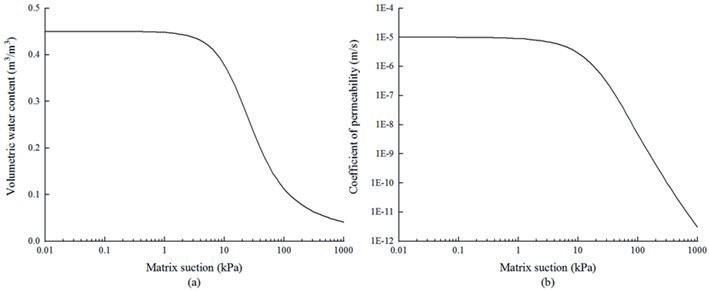
Table 1.
Parameters of silty.
where τ = shear strength of unsaturated soil; c' = effective cohesion; φ' = effective angle of internal friction; σn-σa = net normal stress; σn = total normal stress; σa = pore-air pressure; usually take ua = 0; ua-uw = matric suction; for unsaturated soil, matrix suction equals negative PWP; uw = PWP; φb = the friction angle that varies with the suction of the matrix, called the suction friction angle, which is generally less than φ' and is treated as a constant in SLOPE/W. The strength parameters of silt are shown in Table 1.
Basic Principles of Grey Relation Analysis
(1) Determined the matrices of reference and comparison series and selected the slope stability factors (IPWP, kr, hw and φb) as the comparison series X; take the slope safety coefficient corresponding to each factor as the reference series Y and list the corresponding matrices of X and Y, such as:
(2) Since the physical meaning of each influencing factor in the matrix is different and its magnitudes may be different, they are not comparable with each other or the final results obtained are not accurate enough, so it is necessary to dimensionalize the data in the matrix. The commonly used methods are initialization, mean value, interval relativization, and normalization. In this paper, interval relativization was chosen, such as:
At the same time, do the same for the matrix Y and then obtain the dimensionless matrices X' and Y'.
(3) Determined the difference in information space of the matrices and calculated the corresponding elements in matrices X' and Y'.
then selected maxΔmn and minΔmn in the matrixΔmn.
(4) Calculate the correlation coefficient matrix and the degree of correlation, where the correlation coefficient fmn represents the value of the degree of correlation between the comparison series and the reference series, the value of which is expressed as follows:
where η is the resolution factor and takes values in the range [0,1], generally taking η = 0.5.
In addition, in order to avoid not facilitating holistic comparisons due to the large number of correlation coefficients, the average of the correlation coefficients is used as a quantitative representation of the degree of association between the comparison and reference series, i.e., the correlation degree λm, with the following formula:
The range of relational values is [0,1]. The degree of association between the research object and the influencing factor is mainly described by the order of the correlation degree size, not only the size of the correlation degree value, because the correlation degree size will change but the correlation order does not necessarily change when the number series processing method used in the correlation analysis is different. The larger the correlation value of the influencing factor, the greater the influence of the influencing factor on the slope safety factor, that is, the greater the sensitivity; conversely, the less sensitive.
Slope Model
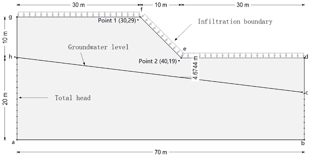
The slope model selected in this paper was taken from the literature [19], The model is 70 m long and 30 m high, the slope height is 10 m, the slope ratio is 1:1, the horizontal distance of the slope is 10 m, and the initial groundwater level height hw = 5 m. The boundary conditions for seepage analysis are as follows: (1) ha and cb are fixed head boundaries, and the head height is the elevation of h and c points, respectively; (2) the bottom edge of the slope ab, and both sides cd, gh are impermeable boundaries; (3) d-g is the infiltration boundary. When the soil permeability is less than the rainfall intensity, part of the rainwater will be lost, and the slope surface will produce runoff. At this time, for the fixed water head boundary, the head height is the ground elevation. When the rainfall intensity is less than the soil permeability, the infiltration boundary is the flow boundary, and the value equals the rainfall intensity. Point 1 (30,29) and Point 2 (40,19) are selected as monitoring points for the change in the seepage field of the slope under the effect of heavy rainfall, as shown in Fig. 2.
Calculation Scheme
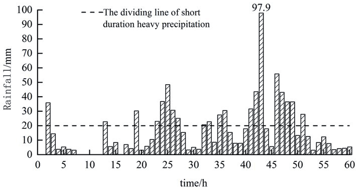
The slope infiltration analysis is generally divided into two parts: first to obtain a steady state analysis of the initial pore water pressure on the slope in order to obtain a pore water pressure closer to the natural state. This method is used to obtain different initial pore water pressure conditions by applying different rainfall intensities to the rainfall boundary. The second is a transient analysis of the rainfall infiltration process. In this paper, the rainfall conditions are the 60 hours of rainfall from 20:00 on the 18th to 08:00 on the 21st monitored at the Zhengzhou Xinmi Baizhai station during the “7.20” exceptionally heavy rainfall disaster, as shown in Fig. 3 [20]. The total amount of rainfall was 985.2 mm, and the number of short-time intense precipitations was as high as 20, with a phased distribution and a maximum rainfall intensity of 97.9 mm/h. The values of four influencing factors, including initial pore water pressure, soil permeability coefficient anisotropy kr, groundwater table height hw, and suction friction angle φb, were taken as shown in Table 2. When the sensitivity of each factor was analyzed using gray relation analysis, the benchmark values were: IPWP = -126 kPa, kr = 1, hw = 5 m, and φb = 26°.
Table 2.
The value of each influencing factor.
Results and Discussion
Changes in Pore Water Pressure
Fig. 4 shows the P1 and P2 pore water pressure rainfall ephemeris curves for the change in initial pore water pressure. Here, the change in initial pore water pressure is achieved by applying a smaller flow boundary to the slope surface. As P1 and P2 are located 1 m below the top and foot of the slope, respectively, their pore water pressures are higher than the set initial pore water pressure minimum, and the pore water pressure response time during rainfall also shows a certain lag. From Fig. 4a), the smaller the initial pore water pressure of P1, the faster the pore water pressure growth rate during the rainfall process; however, after the 28th hour of rainfall, the pore water pressure change trend of P1 is the same under all working conditions. This is because the smaller the initial pore water pressure, the greater the corresponding soil matrix suction, the greater the permeability of the soil, and the faster the pore water pressure growth rate. From Fig. 4b). It can be found that compared with P1, the initial pore water pressure of P2 is larger, and the growth rate of pore water pressure is basically the same as that of P1, but the growth rate of P2 is slower, mainly because P2 is closer to the groundwater level and is greatly affected by the groundwater level, the soil saturation is higher, and the infiltration capacity is weaker. With the rainfall, the groundwater level gradually rises, and when the infiltrating rainwater intersects with the rising groundwater, the pore water pressure of P2 shows a brief sudden change, forming a temporary saturation zone at P2, at which time the pore water pressure of P2 is greater than 0. Later, the temporary saturation zone continues to expand under the action of rainfall, so that the pore water pressure of P2 continues to increase.
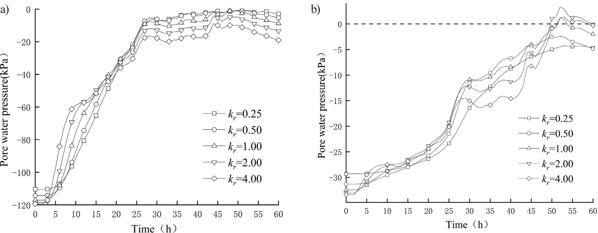
Fig. 5 shows the pore water pressure-rainfall ephemeris curves of P1 and P2 when the permeability anisotropy kr varies. The larger the kr is, the smaller the initial pore water pressure of P1 is, but the decreasing range is not large; in the pre-rainfall period, the larger the kr is, the faster the pore water pressure of P1 and P2 rises, because the larger the kr is, the greater the infiltration coefficient in the y direction, the deeper the rainwater infiltration depth, and the more rainwater infiltration at the same time, the faster the growth of pore water pressure on the slope. When h = 21, the pore water pressure of each working condition is basically the same, but the rainwater has to infiltrate downwards, so the larger kr is, the lower its pore water pressure value is. P2s initial pore water pressure is lower than that of P1, and the growth rate of pore water pressure during rainfall is also lower, mainly because it is closer to groundwater and the pore water pressure is higher under the action of groundwater, resulting in the infiltration coefficient in the y-direction not affecting the initial pore water pressure as significantly as P1. In addition, as P2 is located directly below the foot of the slope, its rainwater infiltration mainly comes from the y-direction, so when kr is small, its pore water pressure growth rate is relatively gentle; however, as kr gradually increases, rainwater infiltration increases and a transient saturation zone is formed at P2.
Fig. 4.
P1 and 2 pore water pressure-rainfall ephemeris curves when the initial pore water pressure changes. a) is a curve diagram of changes in different pore water pressures at position P1. Pore water pressures increase rapidly in the process of rainfall, and the changes tend to be consistent after 28 h. b) shows the variation curve of different pore water pressures at P2. The pore water pressure is larger at the initial stage but increases slowly; it suddenly changes briefly under the action of rainfall and then continues to increase.
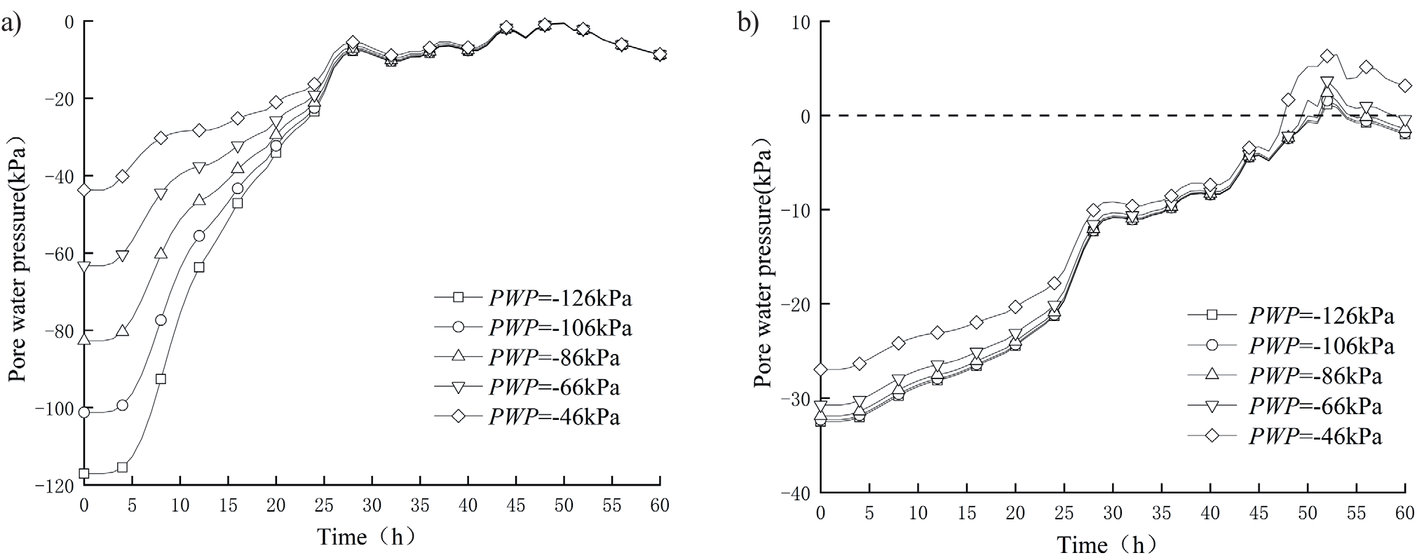
Fig. 5.
P1 and 2 pore water pressure-rainfall ephemeris curves when the coefficient of permeability anisotropy kr changes. a) shows the change curve of pore water pressure at P1 under different permeability anisotropy coefficients kr. The larger the kr, the smaller the pore water pressure at P1. With the increase in rainfall, the pore water pressure in 21 h is basically the same. b) shows the change curve of pore water pressure at P2. The smaller kr is, the slower the growth rate of pore water pressure at P2. With the increase in kr, rainwater infiltration increases, and a transient saturation zone is formed at P2.
As can be seen from the analysis of Fig. 4 and 5, there are some differences in the pore water pressure variation patterns between the monitoring points at the top and bottom of the slope. In addition to the different influencing factors mentioned above, the distance between the monitoring points and the water table is also different. Fig. 6 shows the P1 and P2 pore water pressure-rainfall ephemeris curves as the water table height hw varies. The initial pore water pressure of P1 increases with the increase of hw, and for every 2 m decrease in hw, the initial pore water pressure of P1 decreases by about 18~19 kPa. From Fig. 6b), it can be obtained that the initial pore water pressure of P2 is significantly higher than that of P1, but as hw decreases, its initial pore water pressure changes by the same magnitude as that of P1. During the rainfall process, the higher the hw, the slower the pore water pressure growth rate of P2, and when hw≥7 m, the pore water pressure changes in the same trend in the late rainfall period. It is worth noting that when hw = 3 m, the pore water pressure of the slope increases continuously with the rainfall. This is because when the groundwater level is high, the temporary saturation zone is quickly formed in P2 under the rainfall, after which the infiltrated rainwater makes the temporary saturation zone expand upwards and the pore water pressure increases continuously.
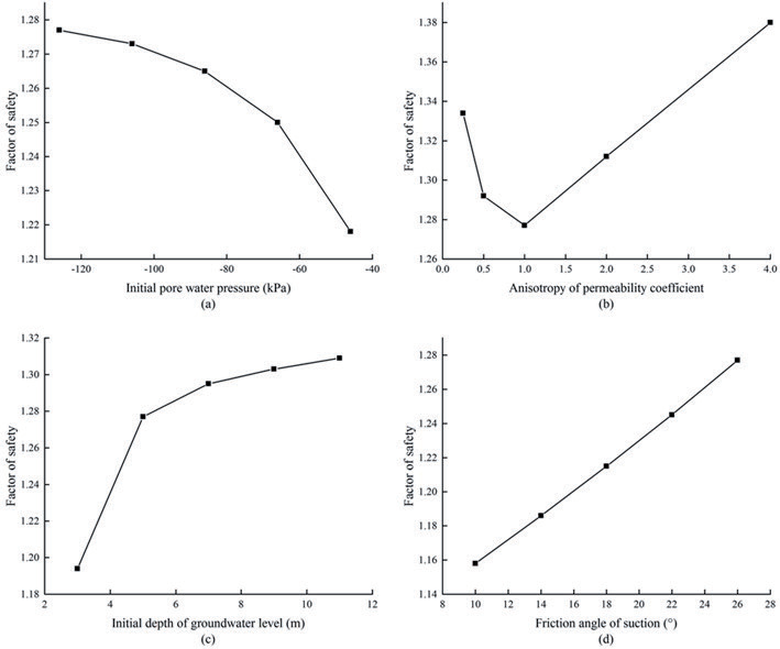
As φb is a shear strength parameter for unsaturated soils, its value is not defined in the SEEP module, and changing its value will not have an effect on the slope pore water pressure; therefore, only the change in the slope safety factor for different φb is analyzed. Fig. 7 shows the relationship between each factor and the slope safety factor at the end of the rainfall. From Fig. 7a), it can be concluded that the greater the initial pore water pressure, the slope safety coefficient gradually decreases, which is because the larger the initial pore water pressure is, the larger the pore water pressure is at the end of rainfall, and the smaller the relative matrix suction, the more unstable the slope is; and for every increase of -20kPa in the initial pore water pressure, the slope safety coefficient decreases by 0.3~2.6%. This is because when kr is smaller or larger, the permeability coefficient in the y-direction decreases or increases, and rainwater cannot infiltrate or infiltrate deeper in the slope in time, resulting in a higher pore water pressure at the slippery surface of the slope, and the corresponding shear strength is higher and the slope is more stable, as shown in Fig. 7b). From Fig. 7c), it can be obtained that the safety coefficient of the slope increases as a logarithmic function with the decrease of hw; the maximum increase of the safety coefficient for every 2m decrease of hw is 6.5% and the minimum is 0.2%, which shows that the higher the water table is, the worse the stability of the slope is; if hw continues to decrease, the safety coefficient of the slope will gradually tend to stabilize and no longer change, which indicates that its influence on the stability of the slope exists at a certain effective distance. As shown in Fig. 7d), the safety coefficient of the slope increases linearly with the increase of φb, and for every 4° increase of φb, the safety coefficient of the slope increases by about 2.4~2.6%. Since its value varies with saturation and is treated as a constant value in SLOPE, its value should be carefully considered in practical engineering applications to avoid large errors.
Fig. 6.
P1 and 2 pore water pressure-rainfall ephemeris curves when the groundwater level height hw changes. a) shows the variation curve of pore water pressure at P1 with different groundwater table heights hw. The larger the hw is, the larger the initial pore water pressure is, and with the gradual increase in rainfall, the change trend is the same at 25 h. b) shows the change curve at P2. When hw is greater than or equal to 7 m, the change trend is the same. When hw is equal to 3 m, slope pore water pressure continues to increase with rainfall.
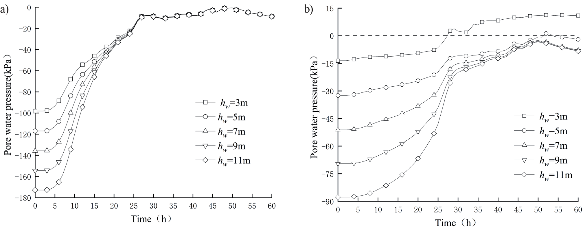
Fig. 7.
The safety factor corresponding to each factor. a) is the broken line diagram of the slope safety factor decreasing gradually with the increase in pore water pressure. b) is a line graph in which the safety factor first decreases and then increases with the increase of kr. c) is a line graph showing that the safety factor gradually increases with the increase of hw. d) is a broken line graph in which the safety factor increases with the increase of φb
Grey Relation Analysis of Slope Sensitivity under Heavy Rainfall
By changing the base value of an influencing factor and keeping the other values unchanged, the PWP data from the SEEP/W module is imported into the SLOPE/W module after the rainfall is over, and then the slope stability under each factor is calculated by the Morgenstern-Price limit equilibrium method. The corresponding slope safety factors Fs for each influencing factor are shown in Table 3.
Based on the data in Table 3, the values of the changes in the influencing factors were used as a comparison matrix for the gray system, and their corresponding safety factors were used as a reference matrix, as follows:
Substituting the above matrix into equation (5) for interval relativization, the resulting dimensionless matrix is then brought into equation (6) to obtain the difference series matrix Δ:
The matrix of Grey relation coefficients can be obtained by using equation (7) as follows:
Finally, the Grey correlation is obtained from equation (8) as: λ = [0.485 0.770 0.760 0.979]T, and the order of correlation is obtained as: φb> kr>hw>IPWP. It can be concluded that of the several factors affecting slope stability under rainfall conditions, φb is the most sensitive to slope stability, followed by kr and hw, and the difference between the two is not significant, with the initial pore water pressure being the least sensitive to slope stability.
Conclusions
Based on the theory of unsaturated soil infiltration and combined with actual rainfall cases, the slope infiltration model of unsaturated silty slopes is established, the infiltration law of the slope under different parameters of each influencing factor is analyzed, the slope stability is studied by the finite element method and the limit equilibrium method, and the sensitivity of each influencing factor is studied by Grey relation analysis. The conclusions are as follows:
(1) The smaller the initial pore water pressure is, the faster the pore water pressure rises on the slope during the rainfall process, but with the growth of rainfall time, the pore water pressure growth rate gradually tends to be the same. The larger the kr is, the smaller the initial pore water pressure is; when kr increases, the pore water pressure at the top of the slope increases faster in the early stage of rainfall, but the pore water pressure at the later stage is lower; the final situation of the pore water pressure at the bottom of the slope is opposite to that at the top of the slope. For every 2m reduction in groundwater level, the slope pore water pressure decreases by about 18~19 kPa; under different groundwater levels, the changing trend of pore water pressure at the top of the slope becomes consistent after the rainfall reaches a certain time; when the groundwater level is high, a temporary saturation zone is generated at the bottom of the slope, and its pore water pressure increases continuously as the rainfall proceeds.
(2) The smaller the initial pore water pressure, the greater the slope safety factor, and for every 20 kPa increase in its value, the slope safety factor decreases by 0.3~2.6%; kr increases or decreases, the slope safety factor increases; hw has a certain effective distance on slope stability, and the maximum change in slope safety factor is 6.5% when hw decreases, and the minimum is 0.2%; φb has a linear relationship with the slope safety factor, and for every 4° increase in its value, the slope safety factor increases by about 2.5%. The slope safety factor increases by about 2.5% for every 4° increase in its value.
(3) The sensitivity of each factor to slope stability is in the following order: φb>kr>hw>IPWP, where the difference between kr and hw is small. It can be seen that for unsaturated soils, the soil strength parameter is also sensitive to slope stability.

