

Introduction
Currently, global ecological issues are of universal concern. Environmental issues, represented by extreme weather phenomena and global warming, are forcing a transformation of economic production sectors. In the SDGs, responsible consumption and production are the 12th element, while climate action is the 13th element. In other words, economic activities that do not damage the climate environment are considered an important element of the Sustainable Development Goals [1, 2]. Sustainable development is not only a remarkable pursuit for developed countries, but also an important matter to be practiced by developing countries [3]. China is the largest developing country in the world in terms of economic size and also one of the largest energy consumers. Since 2018, China has steadily ranked first in the world in terms of carbon emissions, with a huge population, booming transportation, and a massive manufacturing sector contributing to this situation. Because of this, China is facing a serious ecological challenge. The Chinese government has made a corresponding commitment to “climate action”, or carbon peaking, i.e., no further growth in carbon emissions after 2030. The Chinese government is well aware that relying on policy instruments alone to control the scale of production will only slow the growth of carbon emissions, which will not achieve the ultimate goal of carbon neutrality [4]. For this reason, it is necessary to increase the desired output in industrial production as soon as possible. The Chinese government is committed to creating an industrial system of clean production [5]. Compared to the economic value-oriented development model of the past, the Chinese government prefers to consider the overall benefits of industry, especially the ecological contribution of the industry itself. Whether or not there is a negative impact on the environment has become a necessary condition for assessing the industry’s prospects. At the same time, the Chinese government is seeking any means that might be effective for economic transformation or cleaner production. In other words, ecologically oriented industrial transformation is an imminent task for China to consider, and the digital economy is a very favorable tool [6]. Increasingly sophisticated communication technologies have triggered a wave of digital economies, and the digitization of some traditional industries in particular has boomed. The Chinese government favors this economic model with data elements at its core and sees it as a new engine for economic growth. The digitization of industry is the most intuitive manifestation of the digital economy, and decision-making departments often rely on data computing, data analysis, and data forecasting to guide manufacturing activities. However, rapid digitalization is strictly difficult, and the vast majority of industrial companies do not have sufficient budget to invest in driving the digitalization process in their industries. This has given rise to a large number of companies engaged in data services and data computing, whose main business is the analysis and prediction of data, which is known as data industrialization. The emergence of these companies related to the data element has rapidly led to the spread of artificial intelligence among enterprises and a fundamental change in some of the traditional production methods of the past. These companies are also reaching out to other traditional industries through an “embedded” approach, leading to changes in other industries [7].
Needless to say, the Chinese government is very determined in its ambition to achieve green development, and getting rid of environmental regulations and creating a thriving digital economy is a new option for China’s industrial transformation. As a result, a great deal of research has been discussed around the digital economy and environmental development. Several studies have analyzed the relationship between the digital economy and environmental pollution. It was found that the digital economy can effectively reduce air pollution, especially by controlling PM2.5 concentrations and greenhouse gas emissions [8]. Although most of the studies found that the pathways of the digital economy on air pollution are not exactly the same, they are persuasive, at least in terms of their conclusions [9]. In addition to this, the digital economy has a positive effect on sustainable development as well as cleaner production, where the digital economy saves most of the resources by adjusting the allocation of resources while reducing unnecessary links to control the production of non-desired outputs [10]. There are also findings that demonstrate the dynamics of the relationship between the digital economy and ecological sustainability: although the infrastructure of the digital economy increases energy consumption, over time this negative effect is replaced by an increase in production efficiency [11-13]. In other words, in the long run, the digital economy can effectively increase the efficiency of natural resource utilization and improve the quality of the environment, a finding validated in the Chinese sample [14-16]. In the energy sector, the boom of the digital economy has also contributed to the optimization of the energy consumption structure. Specifically, digital technologies have made business production consumption-oriented, increasing the share of effective production in total output and saving energy consumption [17, 18]. In the production sector, the digital economy undoubtedly contributes to the transformation of the industrial structure and plays a stronger role, stimulated by patent regulation and environmental regulations [19, 20]. These studies discuss the relationship between digitization and pollutants in economic production and also analyze the relationship between digitization and the structure of production sectors. However, few studies seem to focus on the impact of exogenous shocks in digitization, a new technological factor, on the efficiency of traditional factor inputs and outputs. So, what is the relationship between the data factor, a non-traditional technological factor, as an exogenous environmental factor, and changes in green total factor productivity?
In this study, we examine the relationship between digital economic development and green total factor productivity using panel data for 247 cities in China over the period 2011 - 2019. The 247 cities selected have a sufficient population and some industrial bases. Some cities that are located in western China are sparsely populated or predominantly agricultural, and are not considered in the scope of this paper. The marginal contributions of this paper may be as follows: First, green total factor productivity (GTFP) measurements have been mentioned a lot in many past studies, and in fact, with the updating of data and refinement of methodology, GTFP has been effectively used in green production. However, many past measures would consider green total factor productivity in isolation, i.e., statistically. At the same time, multiple constraints are not strictly considered in the construction of the indicators; therefore, we provide a new and more realistic way of measuring that has more rigorous results. In addition, in the discussion of mechanisms, we summarize and validate similar findings from past studies. Fortunately, these conclusions still hold under the more stringent GTFP state. Some past studies have argued that the digital economy can promote environmental performance or improve eco-efficiency, while others have found that the digital economy can promote industrial restructuring, and the same is validated, especially from the micro perspective of firms. Therefore, studies that validate the growth of the digital economy in the urban industrial sector can reinforce these arguments. At the same time, we emphasize the important role played by green technologies in this process, i.e., the moderating effect and the threshold effect hold true at the same time, which clarifies the path between the digital economy and the green transformation of industry.
Literature Review
The Literature Context of the Digital Economy
The digital economy was not clearly defined at the beginning, and was used to refer to the new economic relationships made possible by Internet technology. However, with the continuous development of information and communication technologies, the public gradually became aware of the transformative impact of the Internet on economic activities [21]. A growing number of researchers want to give it a precise definition. Over the past two decades, some studies have considered the digital economy as the electronification of the process of trading goods, while others have considered it the online interconnection of business organizational forms [22, 23]. In recent years, when global communication interconnection was commonly achieved, Balcerzak summarized past research and gave a broader definition. He believes that all economic activities driven by ICT can be considered part of the digital economy [24]. A large number of studies on the digital economy now agree that the core of the digital economy is the data element. That is, economic activities that are organized and realized by using information elements by means of information technology [25, 26]. However, there are currently no official digital economy standards issued by the Chinese government. Researchers have developed a number of measurements around the definition and connotation of the digital economy. Jiang et al. provide one of the most direct ways to measure the digital economy, which is to use the ratio of Internet users in the population as a proxy for the digital economy [27, 28]. However, as Internet penetration grows, the growth elasticity of this ratio will become less and less, eventually converging infinitely to 1 (this is, of course, in an ideal state). This seems inconsistent with the real situation of the development of the digital economy. Shahbaz et al. used the entropy method to measure the digital economy index in four areas: infrastructure, social impact, digital trade, and social support, which more fully reflect the areas covered by the digital economy [29]. And the full array polygon graphic index method was used to measure the digitization level in the study by Ren et al. Of course, there are also studies that use the Entropy-TOPSIS model to construct a digital economy model from both input and output perspectives. It mainly covers four aspects of digital innovation elements: digital infrastructure, digital enterprise development, and enterprise digitalization [30, 31]. In addition, some scholars have constructed a digital economy index using the number of Internet users, the number of cell phones used, and the Beijing University Financial Inclusion Index. In general, these digital economy indices measure different forms, but they are all in line with the standard in the selection of indicators [32].
Green Total Factor Productivity
In the beginning, total factor productivity (TFP) was considered a measure of technological progress in production. The DEA model is the most common method to measure TFP. DEA, as a non-parametric technical efficiency analysis method, has been widely used in many social science research fields by virtue of its many advantages, such as no assumption of production function, no strict requirements on the scale of input-output indicators, and the ability to distinguish desired output from non-desired output [33]. Then, in the traditional total factor productivity model, labor, capital, and energy are the basic input variables, while economic output is quite naturally the output variable. However, such a consideration ignored harmful outputs and failed to take note of changes in the external environment [34, 35]. In fact, the energy input is not unlimited, and the carrying capacity of the external environment changes with the scale of production. Based on this situation, scholars have included the factor of environmental pollution in the total factor productivity model, which is the green total factor productivity (GTFP). It is clear that most of the efficiency decreases after considering environmental pollution, which shows that environmental pollution is a factor that should not be neglected, especially in the field of industrial production [36, 37]. Because of this, in order to measure GTFP, researchers have used a large number of different methods to characterize it. In addition to the differences in calculation methods, there are also significant differences in metrics. We will analyze their advantages and disadvantages in detail, as well as emphasize the advantages of using the model in this paper, in Experimental Procedures.
Digital Economy and Green Development
There has been a lot of literature surrounding the digital economy (or ICT industry) and green development in the past, which discusses various impacts of the digital economy and its environmental effects, sustainability, etc. Most of the studies conclude unanimously that there are potential positive benefits of the digital economy on environmental quality on a long-term scale. For example, it has contributions in areas such as improving energy efficiency, reducing greenhouse gas emissions, and enhancing resource management. Thus, the impact of the digital economy on green development is almost certain. And yet, in the case of industrial production, we need to clarify where the digital economy may be contributing to clean industry. The digital economy is driving its own growth through technological innovations that are quickly being applied to the production process. As a result, the efficiency of resource use is further improved, and energy management and environmental monitoring become smarter. As an example, smart grids and smart transportation road networks effectively advance the construction of smart cities. And the central system can well analyze the real-time data of the whole city, so as to provide a reference basis for more optimal decision-making. When the whole city can function efficiently, then the level of public services will be significantly improved. The cost of public spending for businesses is reduced, and more money can be spent on product development and technological improvements. In addition, in the industrial sectors where production takes place, digital information elements are transmitted much faster. There is virtually no time lost in the transfer of data from the production line to the decision-making department. Producers and managers are linked more effectively. Likewise, production costs are greatly reduced, and companies can then gain a higher profit margin and think about how to develop cleaner technologies. Of course, the positive benefits of the digital economy for the environment are potential, as is the case for green total factor productivity. We were able to speculate through the above series of arguments that the digital economy reduces production costs for industrial firms. But, due to the omission of external environmental regulations, will firms really invest this surplus capital created by the digital economy in clean technology R&D? Then, we need to clarify the causes of the “omission of external regulation”. The Chinese government is resolute in its environmental regulations, as evidenced by strict emission standards. Establishing monthly maximum pollution emissions from enterprises based on industrial output and maximum concentrations of hazardous substances in emissions can effectively limit the damage caused by these wastes to the environment. However, it seems that it is easier for companies to acquire equipment to treat wastewater and waste gases than to develop a new production technology. The rewards of technology development are uncertain, but proven waste disposal equipment is practical. Therefore, as long as pollutant emissions are guaranteed to meet standards, companies seem to be more willing to expand production than clean technology development. So, it is true that pollution from industry has decreased, but the change in green total factor productivity is not necessarily due to green technological innovation. We want to measure the true production of industrial firms through green total factor productivity. To this end, we use green technological innovation as a mechanism variable to examine whether the impact of the digital economy on green total factor productivity receives the impact of green technological innovation. So, we need to address three main questions in this study. To this end, we have formulated three hypotheses:
H 1: The development of the digital economy can have a significant impact on GTFP.
H 2: Green technological innovation can moderate the impact of the digital economy on GTFP.
H 3: Green technological innovation acts as a threshold variable in this process.
Experimental Procedures
Measurement of Green Total Factor Productivity
The SBM-DEA Model
As mentioned in Green Total Factor Productivity Section, there are various ways to measure GTFP. It is necessary to compare the different points in common DEA models and analyze their application scenarios. The advantages, disadvantages, and characteristics of various models of DEA are summarized by Ge et al. [38]. Here, we briefly introduce the model chosen in this paper and how it differs from other models. Traditionally, DEA models can be divided into radial and non-radial models. Radial models, represented by CCR and BBC, overlook the issue of slack variables [39, 40]. Moreover, traditional DEA models assume that higher outputs lead to higher efficiency, but they neglect the emissions of environmental pollutants such as SO2 or CO2, which are considered undesirable outputs that cannot be avoided in production activities. Therefore, in addition to maximizing desirable outputs, it is necessary to minimize the generation of undesirable outputs. Traditional DEA models are no longer suitable for handling such undesirable outputs. To address these issues, Tone proposed a slack-based measure (SBM) DEA model, which takes into account the problem of slack variables and avoids underestimating efficiency values. Based on this, Tone further introduced the super-efficiency SBM-DEA model to effectively deal with the problem of no further comparisons being possible after reaching optimal efficiency. Meanwhile, Cooper et al. proposed an SBM-DEA model that considers undesirable outputs [41, 42]. Building on Tone and Cooper et al., the formula demonstrates the SBM-DEA model considering undesirable outputs under the assumption of constant returns to scale (CRS):
Assuming there are n decision-making units, m inputs, S1 desirable outputs, and S2 undesirable outputs, the input matrix is denoted as X = [x1, ..., xn]∈Rm×n, the desirable output matrix as Yg = [y1g, ..., yng]∈Rs1×n, and the undesirable output matrix as Yb = [y1b, ..., ynb]∈Rs2×n. It is also assumed that X>0, Yg>0 and Yb>0. Therefore, the production possibility set P̃, which includes undesirable outputs, is defined as follows: P̃ = {(x, yg, yb)|x≥Xλ, yg≤Ygλ, yb≥Yb, λ≥ 0}, where λ∈Rn is the intensity vector. This production possibility set with undesirable outputs is defined under the assumption of CRS.
Where s–∈Rm represents input excess (input slack variable), sb∈Rs2 represents excess production of undesirable outputs (undesirable output slack variable), and sg∈Rs1 represents production shortfall of desirable outputs (desirable output slack variable). The objective function ensures that si–(∀i), srg(∀r), srb(∀r)strictly decrease. The optimal solution of the objective function is denoted as
The DEA-SBM-ML Model
Traditional efficiency measurement methods are limited to static comparative analysis, making it difficult to capture changes in the production process over time. However, in reality, technology is constantly evolving. To address this issue, Färe et al. proposed the Malmquist Productivity Index (MPI) to measure the changes in decision-making units between two periods [35]. Pastor and Lovell further introduced the Global Malmquist Index (GMI), which considers data from all periods and treats them as a holistic productivity possible set (PPS).
Assuming that the reference sets for each period are denoted as Sg, we have Sg = S1 ∪ S2 ∪ S3 ∪ ... ∪ SP. GMI solves two problems: the possibility of infeasible solutions under the variable returns to scale (VRS) assumption and the lack of transitivity [43]. Previous studies have often built the GM index on the Directional Distance Function (DDF) [34]. However, the choice of direction vectors is subjective. Therefore, in this study, we continue to construct the GM index within the SBM model, considering undesirable outputs. Thus, the calculation of total factor productivity is transformed into the Green Global Malmquist-Luenberger Index, represented by the following formula:
In the given context, (xt, yt, bt) and (xt+1, yt+1, bt+1) represent the inputs, desirable outputs, and undesirable outputs in period t and period t+1, respectively. Et and Et+1 represent the technical efficiency of input and output for the production technology at times t and t+1. TC denotes the measure of technological change, and EC represents the measure of efficiency change. When the global reference-based Malmquist-Luenberger value is greater than 1, it indicates an improvement in productivity. When the productivity value is less than 1, it represents a decrease in productivity. A productivity value of 1 indicates no change in productivity. In other words, the ML index is able to reflect the technological progress of each year. Unfortunately, this efficiency is calculated based on the previous year’s base period. That is, it cannot measure the change in efficiency over multiple consecutive years. For this reason, we performed a cumulative multiplication process using 2011 as the base period to examine the change over the period 2011-2019 [44, 45].
Selection of Indicators for the DEA Model
Next, we need to consider the components of the Green Total Factor Productivity Index. Certainly, a large number of past studies provide us with good references [46]. Here, the traditional input indicators are still divided into labor, energy and capital. They are measured by the number of employees, the amount of standard coal consumed for energy, and the capital stock, respectively.
And in the expected output part, we take fiscal revenue into consideration in addition to the traditional economic output. Although GDP is regarded as the best indicator of the level of economic development, the composition of its economic output varies greatly from region to region, due to the huge differences in industrial structure, industrial level and openness. For example, there are three cities with exactly the same output value, but one of them relies on plantation, another is reduced to a foreign-owned foundry, and the last one is a headquarters for R&D of high-tech products. Obviously, they do not have the same economic output. However, too many indicators will reduce the accuracy of the measurement results and we cannot figure out this black box. Therefore, we would like to include a suitable indicator to reflect the differences between different cities in addition to economic output. Obviously, fiscal revenue is a suitable choice. If a region has a high GDP and low fiscal revenue, then we should reasonably suspect that the region is perhaps not as industrially advanced as we think.
Finally, there is the non-desired output component. In general, industrial SO2 is considered the most direct undesired output. There are also many studies that consider industrial wastewater, industrial dust, and industrial waste gas as non-desired outputs. However, in this paper, we use data on haze. We hope that the annual average unit concentration of PM2.5 can reflect the pollution status of the region. This data is obtained from the Atmospheric Composition Analysis Group, Dalhousie University, and is more representative of the real situation than some official statistics.
Econometric Models
Baseline Regression: a Panel, Two-Way Fixed Model
To examine the relationship between DE and GTFP, we need to construct a benchmark regression model. Based on the previous study [9], we chose a two-way fixed-effects panel data model. This model takes into account individual differences and time differences, and the regression results are more realistic; see Equation 1.
Here, i stands for individual, and t stands for time. GTFP is shorthand for Green Total Factor Productivity, while DE is the digital economy and C is a set of control variables. u and v denote individual and time effects, respectively, and ε is a stochastic error term.
Confirmation of Impact Mechanisms: Moderating and Threshold Effects
Furthermore, we need to add the moderating variable term to equation 1 to account for the moderating effect of green technological innovation, i.e., Equation 2.
Finally, we need to investigate whether green technological innovation can be used as a threshold variable in the process of the digital economy, affecting green total factor productivity. For this purpose, we constructed Equation (3).
Here, q is the threshold variable, w(.) represents the indicator function with a value of 1 or 0 (if the condition in the brackets is satisfied, then the value is assigned to 1; otherwise, it is 0.), p is the specific threshold value.
Selection of Variables
Explained variable: The dependent variable in this paper is GTFP, and its calculation procedure and method are derived from the Measurement of Green Total Factor Productivity. The explanatory variable, which is the independent variable, is the digital economy index(de). In this paper, based on a large number of previous literature studies, the digital economy index is constructed using principal component analysis. The principal component analysis method has been widely used in studies in similar fields. We selected four indicators, including the number of Internet users per 100 people, the total amount of telecommunication services per capita, the number of cell phone subscribers per 100 people, and the digital financial inclusion index (Peking University). For the control variables, we chose total fiscal expenditures(fe), the number of industrial enterprises above the scale(nie), per capita regional GDP(eco), and the number of residents’ savings(sav). Mechanism variable: The sum of green invention patents and green utility model patents in each region is used to measure green technological innovation(gtec). To alleviate the heteroskedasticity problem, all control variables were logarithmically treated.
Data Sources
In the DEA-SBM-ML model, the number of employees, fiscal revenue, and gross regional product are obtained from the CSMAR Database (of course, some missing values are also filled in from the statistical yearbooks of prefecture-level cities). The number of tons of standard coal consumption is obtained from the China Energy Statistical Yearbook. For the capital stock data, the perpetual inventory method is used to derive results, where the depreciation rate is 10.96% and the base year is 2000 [47]. For the average PM2.5 concentration, publicly available data from the Atmospheric Composition Analysis Group of Dalhousie University was used [48]. In the regression model, all variables and their components were obtained from the CSMAR database, except for green technological innovation, which was obtained from the CNRDS database.
Results and Discussion
First, we compiled the results of the variable measures in Experimental Procedures, as shown in Table 1.
Table 1.
Descriptive statistics of variables.
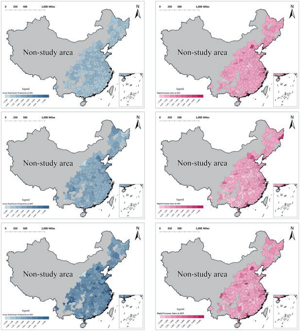
Further, to show more clearly the spatial-temporal variation of the main variables, we plotted Fig. 1. where the left side shows the distribution of gtfp from top to bottom for 2011, 2015, and 2019, while the right side corresponds to the spatial pattern of de. As can be seen from Fig. 1, both de and gtfp are gradually increasing over time. gtfp increases more significantly in coastal areas and inland central cities. As far as de is concerned, de values are usually higher in provincial capitals than in other regions.
To test Hypothesis 1, we conducted a benchmark regression, and the results are shown in Table 2. From the left to the right are the results of regressions, with the gradual addition of control variables. The first column shows the results of the regression without adding any control variables, and the coefficient is 0.406 with a t-value of 5.43, which is significant at the 1 percent level. However, this result is not credible because it suffers from the problem of important omitted variables. After we add other variables that may have an impact on green total factor productivity to the model, we find that the regression coefficients of DE remain around 0.38 and are all significant at the 1 percent level. Therefore, we consider the conclusions to be reliable. In other words, the digital economy can contribute to the growth of GTFP. Next, we also need to briefly focus on the coefficients of the control variables, where nie and sav have a negative effect on GTFP. It may be because the growth in the number of above-scale industries is mainly due to the gradual expansion of some small and medium-sized enterprises (SMEs), which are still immature and therefore not sufficiently advanced in terms of production technology. As for savings, it may be because too much savings will squeeze the factor inputs for innovation and hinder the progress of GTFP. Overall, however, hypothesis 1 was tested.
Next, to ensure the reliability of the experimental results, we need to test the robustness of the regression equations. Therefore, we conducted panel quantile regression as well as 1% and 99% reduced-tail regression. Thus, we use a panel quantile regression model, exclude the exceptional samples, and shrink the tails by 1% and 99% for robustness testing. As shown in Table 3, the first column shows the results of the panel quantile regression at the 90 percent level, the second column shows the results of the panel quantile regression at the 75 percent level, the third column shows the results of the panel quantile regression at the 60 percent level, the fourth column shows the results of the reduced-tailed regression, and the fifth column shows the results after excluding the four special cities of Shanghai, Beijing, Tianjin, and Chongqing.
We find that all the coefficients of de are greater than 0 and remain significant from columns 1 to 5. This indicates that our model construction is robust. Further, we need to consider whether there are important omitted variables that cause the model to be endogenous. In this paper, an instrumental variables approach is used to address this issue. The basic requirement for an instrumental variable is that it is correlated with the inner variable, but must be an exogenous variable. We use the product of the number of telephone subscribers per 10,000 people in each region in 1984 and the number of Internet subscribers in the previous period as the instrumental variable.
Table 2.
Benchmark regression results.
Table 3.
Robustness test results.
As shown in Table 4, it can be seen that the F-value of the first column is greater than 10, P-value is also 0, which indicates that the instrumental variables selected in this paper are not weak instrumental variables. Moreover, the number of instrumental variables and endogenous variables are equal, which indicates that there is no over-identification problem. Then the regression coefficient of iv in the first stage is positive and significant. This indicates that there is a positive correlation between instrumental variables and independent variables. The results of the second stage are consistent with the baseline regression, which indicates that the results are robust. Next, we turn to the issue of regional heterogeneity. Now that Hypothesis 1 has been verified to be reliable, we would like to know whether DE pairs of GTFP will demonstrate different effects in different regions. However, since we have excluded many cities in the western provinces from our sample selection, it would be easier to simply divide the full sample into eastern, central, and western. It may leave the western region with too small a sample. Therefore, we have classified them into three types, namely, high, medium, and low, according to the level of economic development of the districts. Specifically, we calculated the average GDP per capita for 2011- 2020 as an evaluation criterion. We consider areas greater than 60,000RMB (the current price translates to approximately $8,400) as value areas and areas between 33,000-60,000RMB as average areas. Finally, we consider areas below 33,000RMB as low areas (the current price is about $4,600). Table 5 demonstrates the results of the heterogeneity test, where the first column is the low areas, the second column is the average areas, and the third column is the high areas.
We were surprised to find that the effect of DE on GTFP varies widely across regions. The regression coefficient reaches 0.740 in regions with higher levels of economic development, while in regions with lower levels of economic development, the result is only 0.017 and insignificant. This suggests that the digital economy contributes more significantly to green total factor productivity in regions with better economic development, which is a sign of strength. The digital economy can play a more critical role in regions with well-developed industrial systems and high economic development. Conversely, in some lagging regions, its role is limited.
Table 4.
2SLS-IV regression results.
| First stage | Second stage | |
|---|---|---|
| de | gtfp | |
| iv | 0.556*** | |
| (3.73) | ||
| de | 0.523* | |
| (1.77) | ||
| Control | YES | YES |
| Year | YES | YES |
| City | YES | YES |
| N | 2223 | 2223 |
| adj. R2 | 0.425 | 0.321 |
| F | 97.80 |
Table 5.
Results of the heterogeneity test.
At this point, the validation of Hypothesis 1 is essentially over. We need to further analyze the mechanism issue. That is, what are the mechanisms by which the digital economy affects green total factor productivity? Of course, this hypothesis has already been proposed in the previous section, and we would like to examine the role that green technological innovation may play in this process. Therefore, we ran a regression on equation 2, and the results are shown in Table 6.
Next, observe the regression results in Table 6. In order to present a clearer picture of the regression, we report the results without putting the control variables together. In addition, we also place the first and fifth columns from Table 1 here. Note that later in the hypotheses, we need to ensure the stability of the main variable (DE). If the significance of the main variable and the direction of the coefficients change significantly with the inclusion of the interaction term, then the coefficients of the interaction term are meaningless. Fortunately, the direction of the coefficients on all of the main variables remained consistent, suggesting that the addition of the interaction term did not create a new endogenous problem. Then, we observe the coefficients and significance of the two interaction terms, and they are 0.057 and 0.056, respectively. This means that green technological innovation has a positive moderating effect on the digital economy, regardless of whether control variables are considered or not. In other words, the coefficient of DE grows with gtec. In that case, the second hypothesis is also verified. Finally, we want to examine whether green technological innovation acts as a threshold variable in this process. Accordingly, we perform a threshold regression.
Table 6.
Regression results for moderating effects.
We set up 300 Bootstrap tests, performing single-threshold, double-threshold, and triple-threshold tests in that order. The results show that the F-value for the first threshold is 28.42, the F-value for the second threshold is 68.58, and the F-value for the third threshold is 30.60. The P-value is less than 0.1, which suggests that there may be a triple threshold. However, in terms of confidence intervals, the third of the triple thresholds is missing the upper and lower thresholds. This suggests that the third threshold, the one with a threshold value of 8.104, does not exist (this conclusion is, of course, further verified in the LR diagram). Therefore, we believe that there are just two thresholds, which means that this is a two-threshold model. Next, we divided the time period of the study sample into Phase I and Phase II. The first phase covers the period 2011-2015, while the second phase covers the period 2015-2019. Note that 2015 is included in both phases. Of course, again, we need to examine the existence of their thresholds first, and the results are shown in Table 7. Next, we perform threshold regression analyses for the full sample, Phase I, and Phase II, and their results are displayed in Table 8.
Table 7.
Test for number of thresholds.
Table 8.
Tests for Phase I Thresholds and Phase II Thresholds.
To verify that these results are accurate, we plotted the LRs for the full sample, stage 1 and stage 2, see Fig. 2. Not surprisingly, all thresholds are consistent with those in Tables 7 and 8.
The above results indicate that our resulting threshold regression results are plausible. We interpret the results in Table 9. In the full sample area, there are two thresholds for green technological innovation, at 1.390 and 2.468. When the value of gtec is smaller than the first threshold, the regression coefficient of de is only 0.202, while when the value of gtec is between the two thresholds, the regression coefficient of de is 0.420. If the value of gtec exceeds the second threshold, the regression coefficient of de becomes 0.994. It can be said that the difference between the three regression coefficients is still relatively large. Next, we look at the regression results for the first period. We find that the driving effect of the DE on GTFP is insignificant when gtec is smaller than the first threshold. The regression coefficient is 0.411 when gtec is between the two thresholds, and this result is 0.669 when gtec is larger than the second threshold. The overall regression coefficient is lower than that for the full sample period, which is certainly in line with the true picture. This period is in the early stages of the development of the digital economy the concept of green total factor productivity is not yet widely recognized and pollution control in China is still in its infancy. Finally, we observe the regression results between 2015-2019. At less than the first threshold, the regression coefficient is 0.256, after crossing the first threshold, this result comes to 0.437, and after crossing the second threshold, this result becomes 1.020, with all three regression coefficients significant. This result is similar to the full sample, which indicates that the results of the threshold regression are plausible. Note, however, that their thresholds change after distinguishing between the before and after phases (of course, you can easily spot this in Fig. 2). Here, we are looking to examine the existence of the thresholds at different time periods rather than the changes in the threshold values. Because we are using panel data, its experimental results are only responsible for China from 2011-2019. That is, if the data are available, we assume that the interval of the study extends backward from 2019 to 2022 or even 2023, where the results become different. In fact, the reasons for the difference in thresholds are quite understandable. In different time periods, either DE, GTFP, or gtec, their means as well as their statistical distributions are different, and in general, the second stage is slightly higher than the first. From the regression coefficients themselves, the coefficients are relatively higher in the second stage, which suggests that the growth rate of GTFP is higher than that of DE in the second stage. Of course, this is literally true. What we are trying to convey is that the thresholds are not likely to be uniform because of the stochastic nature of the movement of the mechanism variable, the independent variable, and the dependent variable. But one thing can be proved: in any case, we are sure that gtec can act as a threshold variable in this interval and that the positive effect of the digital economy on GTFP is stronger when the level of gtec exceeds a specific value. At this point, hypothesis 3 is verified.
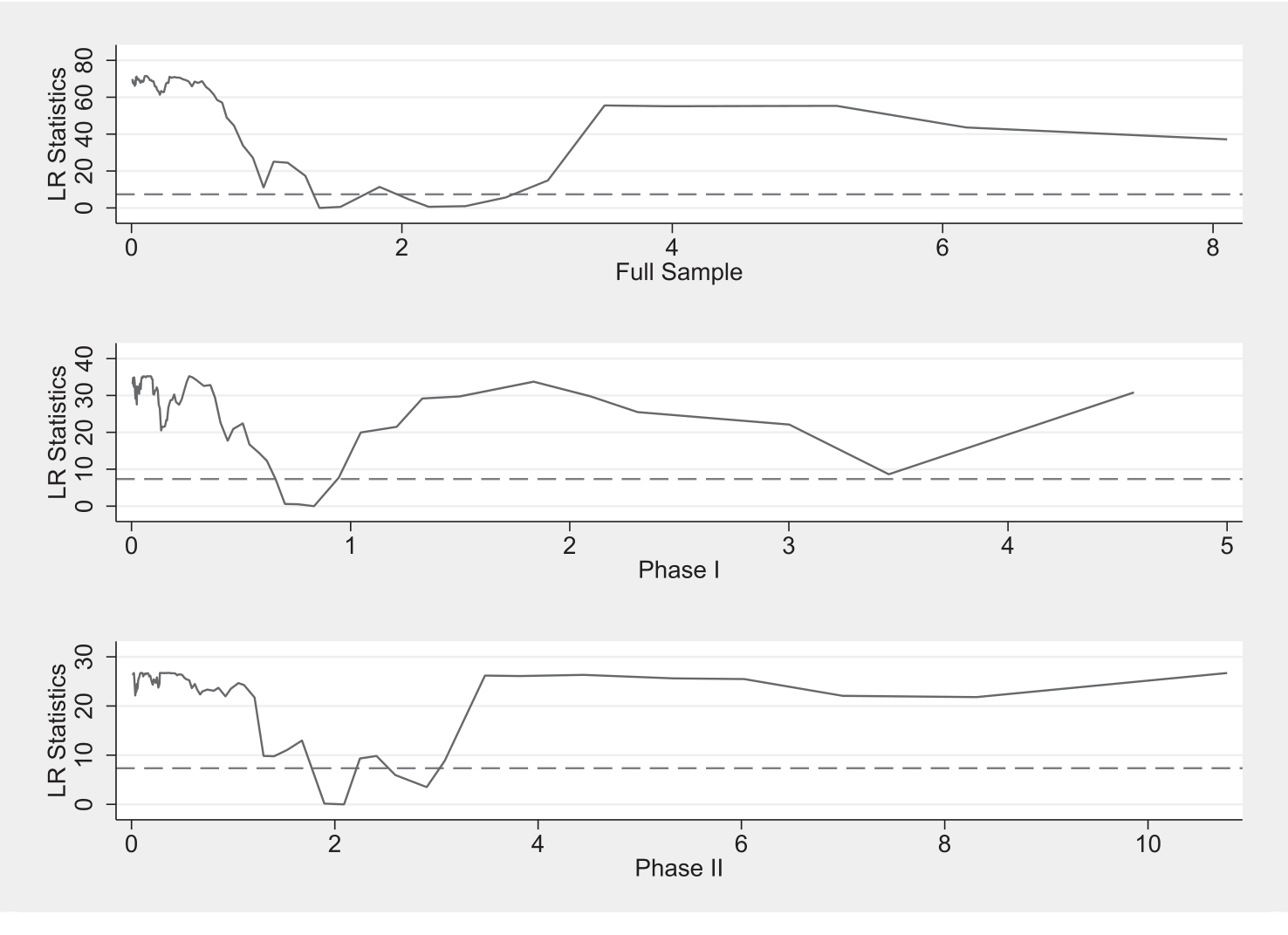
Table 9.
Threshold regression results.
Discussion
In this study, we constructed the DEA-SBM-ML model to measure GTFP. Here, we integrated the non-expected outputs into the model and, unlike the static model, included the ML index. The indicator system here is also relatively more suitable for industrial use. Of course, as we mentioned earlier, the increase in green total factor productivity is not necessarily generated by advances in clean technology. Therefore, we need to fully consider the mechanism of action while examining the impact of the digital economy on green total factor productivity. In this way, we introduced green technological innovation into the regression model and examined the moderating effect and threshold effect. At least from the feedback from the results of this study, we are assured that the green transition caused by the digital economy is transforming the production side. That is, digitization is fundamentally transformative for producers from the production side. And, for the time being, the threshold effect of green technologies is still very much in evidence. Interestingly, we found differences in the impact of the digital economy on the green transition over time. As mentioned in Results, the digital economy had not yet become a popularly recognized form of economy in the early days, and the technological conditions of communication at that time could not satisfy the adoption of digital technology by a large number of vendors, so we consider whether the intensity of the digital economy itself also has some impact on green total factor productivity. Of course, similar conclusions have been proven to be correct in this study [49]. Therefore, our study is basically in line with the existing similar conclusions. In other words, China’s industrial green TFP is in line with urban TFP in terms of the overall trend, which suggests that China’s economic growth is still exported through industrial orientation. Here, we can infer an interesting and unexpected result. The green transformation of China’s industry actually largely determines the degree of China’s green development transformation. How can we understand this conclusion? If there is a significant difference between the changes in industrial green total factor productivity and the changes in green total factor productivity, it indicates that industrial green transformation is ahead of or behind all sectors of green transformation, and the consumption growth pole that the Chinese government is committed to building has already taken shape. However, it has been proven that there has not been a clear differentiation between the two, which has been further confirmed in similar studies. In past studies, scholars have discussed various elements related to the green transition. Our new evidence affirms these findings from the prefecture-level industrial sector and examines the role of the digital economy at different levels, using green technologies as a new discriminant criterion. This adds ample evidence to past research on the digital economy and green development. As previously described, because of our more scientific and precise identification of green total factor productivity, the results are perhaps more rigorously demanded in actual experiments. In particular, with the introduction of the ML index, industrial green production is no longer an independent decision-making unit, and the dynamic model effectively overcomes the shortcomings of the static model. Because industrial production is a continuous and uninterrupted process, the dynamic model is more consistent with the facts. Fortunately, despite our strict constraints on the calculation of green total factor productivity, the digital economy still shows positive effects.
Of course, there are some limitations to our study. This is unavoidable, but we hope that these limitations will provide new research directions for future work. Although we have pinpointed our study to the green transformation of the industrial sector in urban China, cities are still a larger area relative to manufacturers. Due to data limitations, we are unable to examine the differences between green total factor productivity across industries. However, such differences may in fact exist, and we believe that there may also be heterogeneity in the facilitating effects of the digital economy on different urban industrial clusters. This is an issue beyond our experimental design. In addition, although the supply side is a part of the functioning of the economy, the fact is that industrial output also affects production to a greater or lesser extent. Therefore, if a dynamic model is used to calculate GTFP, the consumption phase should also be included in the DEA model. Unfortunately, the consumption phase is not well identified by the data. Overall, however, our conclusions are scientifically credible.
Conclusions
All conclusions point to the following conclusions: The rapid development of the digital economy has caused a series of changes in the industrial manufacturing industry, which has effectively promoted the improvement of GTFP in Chinese cities. Our empirical evidence from Chinese cities from 2011-2019 proves that the digital economy can fully serve as the spearhead of China’s “green reform”, and the digital economy plays an important role in this process. Then, we also discuss the role of green technological innovation in this process. We find that an increase in green technological innovation can effectively inflate the role of the digital economy and act as a threshold variable. In layman’s terms, when the level of green technological innovation in a region is high enough, the digital economy can contribute to GTFP more effectively. In the benchmark regressions, we examine regressions in different regions, similar to most past studies. Regions with lower levels of economic development have always struggled to benefit from the rapid development of the digital economy, while regions with higher levels of economic development have often been able to ride the “digital dividend”.
Based on these findings, we can make some recommendations to promote China’s green transition. First, the Chinese government should strengthen the infrastructure of the digital economy, which has brought many real benefits to economic development and has been proven to contribute to China’s green development. In this process, it is necessary to pay attention to the development of the digital economy in some economically underdeveloped regions [50, 51]. We do not expect the digital economy in these regions to catch up with the developed regions, but we do not want to see a wider digital divide. Of course, we also need to pay attention to the development of the industrial enterprises themselves in these regions; otherwise, the digital economy will have little effect on GTFP.
The second point is that as digital technology matures, the cost of digital transformation for enterprises is getting lower and lower. The government can follow the trend and strengthen the subsidization of green finance and other policies to induce enterprises to transform into cleaner production. We are convinced that the level of green technological innovation largely affects the size of the digital economy’s role in GTFP [52-54]. After the abolition of sewage charges in 2018, the Chinese government has fewer direct regulatory tools. Of course, much of this is due to the fact that a portion of the funds are being used to compensate for innovation. In short, encouraging green technological innovation is good for both the digital economy and green total factor productivity [55].
Thirdly, we should also see that many factors influence GTFP in different regions and at different times. These factors are both positive and negative. This shows that the digital economy can have different effects in different regions. This requires local governments to make corresponding adjustments according to their own situation when facing the central government simulation. China’s development has obvious stages, and the biggest imbalance in China is seen between regions. Such an imbalance is shown in time and space [56]. Therefore, how to utilize the digital economy is a major issue that local governments need to think deeply about. In particular, when dealing with some investment projects, these local governments should give due consideration to revenue returns. While such investments could be seen as transformational funds for green development, it is important to consider the limited nature of the returns, and they should not blindly develop the “digital economy” in isolation from the actual situation, nor should they see it as a new opportunity to enhance their status [57].

