

Introduction
The greenhouse effect, primarily driven by carbon emissions, leads to various environmental problems, including global warming, climate change, acid rain, and ozone layer depletion [1]. These issues significantly impact water and food resources, energy production and consumption, ecosystems, human health, and overall economic and social well-being [2, 3]. Nitrous oxide (N2O) is nearly 300 times more potent than carbon dioxide (CO2) in terms of the greenhouse effect and contributes to severe air pollution, especially in agricultural regions [4, 5]. At the 26th United Nations Summit on Climate Change in 2021, Vietnam joined 150 other countries pledging to reduce CO2, N2O, CH4 (methane), and CFCs (chlorofluorocarbons) emissions to achieve net-zero carbon emissions by 2050 [6]. The Vietnamese government has committed to these goals through various strategies, including the “National Strategy on Climate Change to 2050”, which outlines comprehensive tasks and solutions for implementing COP26 commitments [7, 5]. Moreover, several management activities have been undertaken to achieve the net-zero carbon emission targets, including low-carbon technology innovation, natural resource mobilization, and economic relationships [8, 9]. Despite these efforts, Hanoi, the capital of Vietnam, was ranked fourth in the world in terms of the worst air quality in 2022 [10].
The relationship between greenhouse gases and socioeconomic factors such as foreign direct investment (FDI), gross fixed capital, economic growth, trade openness, energy consumption, and industrial growth has garnered significant interest from researchers and policymakers [11, 12, 4]. The Environmental Kuznets Curve (EKC) hypothesis, introduced by [13], suggests a nonlinear relationship between environmental quality and economic growth, with emissions initially rising and then declining after a certain income threshold is surpassed. Multiple investigations conducted by researchers and documented in various studies have explored the validity of the EKC hypothesis through experimental research, mainly employing gross domestic product (GDP) growth as a typical variable of interest and CO2 emissions as the central dependent variable [14]. While some studies support an inverted U-shaped link between environmental quality and economic development [15-19], others have found mixed results [20, 21]. However, many studies have not provided statistical evidence to confirm this hypothesis [22, 23].
Along with GDP growth, financial development plays a crucial role in shaping environmental quality [24]. This encompasses the growth and efficiency of financial markets and institutions and can influence environmental outcomes through various channels. For instance, financial development can facilitate investments in green technologies and infrastructure, support the transition to a low-carbon economy, and enable better management of environmental risks [25, 26]. Moreover, it can enhance access to capital for businesses and individuals, promoting sustainable practices, social contributions, and innovations that reduce emissions and environmental degradation [27-29]. However, the relationship between financial development and environmental quality is complex and multifaceted [24]. While financial development can drive economic growth and improve environmental standards through technological advancements and efficient resource allocation, it can also lead to increased industrial activities and higher emissions if not managed appropriately [30]. This duality underscores the importance of understanding the nonlinear effects of financial development on environmental quality, particularly in developing countries such as Vietnam, where economic and environmental priorities often intersect [31, 32].
Despite extensive investigations, significant research gaps remain. Notably, there is a scarcity of studies focusing on the nonlinear effects of financial development on environmental degradation in Vietnam, particularly using updated time frames and comprehensive control variables. Existing research in Vietnam often emphasizes economic growth, missing the underexplored impact of financial development owing to its complicated relations. Moreover, the use of advanced econometric models such as the Autoregressive Distributed Lag (ARDL) bound test model, which can handle small sample sizes and address endogeneity issues, has been limited. This study aims to address these gaps by examining the nonlinear influence of financial development on pollutants such as CO2 and N2O emissions in Vietnam over an updated period from 1990 to 2021. Furthermore, limited research has explored the combined effects of the EKC and Pollution Haven Hypothesis (PHH), considering the impact of FDI and international trade on environmental quality. This study incorporates both hypotheses to provide a more comprehensive analysis of the factors influencing environmental quality in Vietnam. Additionally, the inclusion of N2O emissions as a dependent variable broadens the EKC perspective and highlights the significant role of agricultural practices and industrial activities in greenhouse gas emissions.
Country-specific studies are vital due to the heterogeneous nature of different countries. Each country differs in terms of institutions, economic growth, and pollution. Thus, this study examines whether the EKC exists in Vietnam. The main findings are summarized as follows. Dynamic ARDL simulations revealed a U-shaped relationship between financial development and greenhouse gas emissions (CO2 and N2O) in Vietnam, indicating that while financial development may initially improve the environment, it can deteriorate after a certain stage. The influx of FDI was found to reduce both CO2 and N2O emissions, ensuring the invalidity of the PHH in Vietnam. Trade openness has a detrimental impact on CO2 emissions but not on N2O emissions, suggesting that the environmental impact of trade openness depends on the sectoral composition of a country’s trade. Gross fixed capital formation and industrial development increased both CO2 and N2O emissions, whereas energy consumption significantly increased CO2 emissions but did not affect N2O emissions. The short-term estimates revealed that the effects of various factors on CO2 and N2O emissions differed, with financial development, trade openness, and energy consumption having varying short-term impacts on these two pollutants. The findings also support the existence of a long-term relationship among the relevant variables and highlight the importance of considering both short- and long-term impacts when assessing the relationship between economic factors and environmental degradation. These findings highlight the complex dynamics between economic activities and environmental outcomes and inform policy decisions aimed at balancing economic growth and environmental sustainability.
The remainder of this paper is organized as follows: Section 2 presents a review of the relevant literature. Section 3 outlines the empirical model, methodological strategies, and data collection method. Section 4 discusses the findings of the study. Concluding remarks and policy implications are presented in the final section.
Literature Review
The EKC hypothesis posits an inverted U-shaped relationship between environmental degradation and economic growth, in which initial economic growth leads to increased environmental degradation; however, after a certain level of income per capita is reached, further growth results in environmental improvement [13]. The development of financial institutions and markets plays a crucial role in economic growth by improving the efficiency of the financial system [33]. It enables households and companies to access capital and credit at minimal cost, facilitating wealth creation and ultimately driving economic growth [34]. Well-developed financial markets enhance resource allocation efficiency, facilitating increased investments in environmentally friendly technologies and sustainable practices, and financial markets enable firms to invest in cleaner technologies and innovations by providing access to capital, thereby reducing pollution and improving environmental quality [35-37]. Furthermore, financial institutions play a crucial role in funding firms to adopt environmentally sustainable technologies, influencing the shape of the different EKCs [38-40]. However, financial development lowers barriers for investors by providing easier access to capital, which encourages new capital investments. This increase in investments often leads to a higher consumption of energy resources, resulting in greater greenhouse gas emissions [41, 33]. Thus, the relationship between financial development and environmental quality is considered nonlinear [42]. This duality underscores the complexity of the relationship between financial development and environmental quality. While financial development can drive economic growth and technological advancements that enhance environmental standards, it can also result in an increase in industrial activities and higher emissions if not adequately managed, aligning with the PHH when financial institutions primarily fund pollution-intensive industries in countries with lax environmental regulations [39, 43, 44]. This highlights the need for a thorough investigation to ensure that financial development contributes positively to environmental sustainability.
Thus, this study aims to examine the nonlinear effects of financial development on environmental degradation in Vietnam to address existing research gaps, including the exploration of the short- and long-term relationships between financial development and environmental quality. Additionally, this study incorporates both the EKC and the PHH to provide a more comprehensive analysis of the interplay among financial development, foreign direct investment, international trade, and environmental outcomes in Vietnam.
Relationship between Environmental Quality and Financial Development
CO2 emissions have emerged as a critical focal point in environmental research owing to their significant impact on climate change and global warming [45, 46]. The persistent relationship between financial growth and CO2 emissions has been widely studied, highlighting the complex interplay between economic activities and environmental sustainability. [42] found an inverse U-shaped relationship between financial development and CO2 emissions in Malaysia. In the long term, financial development contributes to a reduction in CO2 emissions but is associated with increased CO2 emissions in the short term. According to [47], the system-generalized method of moments regression was applied to panel data from 1990 to 2013. Their findings suggested that financial development has the potential to mitigate long-term environmental degradation in 19 emerging economies through investments in green technologies and energy efficiency. [48] assessed the influence of financial development on CO2 emissions in 11 European Union countries from 1995 to 2017. Financial development can lead to positive environmental outcomes, depending on how financial resources are utilized, such as industrial activities and higher energy consumption. [49] confirmed that the EKC applies to the relationship between environmental degradation and financial development in the Asia-Pacific region. Their findings indicated a nonlinear relationship between financial development and CO2 emissions, consistent with the EKC hypothesis in the Asia-Pacific region. [11] found that the overall effect of financial development on CO2 emissions was influenced by economic growth and renewable energy consumption in 148 countries from 1990 to 2019. The impact of financial development on environmental quality varies according to the income group. The positive role of renewable energy consumption in reducing CO2 emissions is significant in high- and middle-income countries.
Financial development can lead to increased industrial activities, higher energy consumption, and consequently, greater environmental degradation [50, 51]. However, it also potentially facilitates investments in cleaner technologies and energy-efficient processes [52]. The conclusions of [53] and [54] are in contrast with those of previous studies on the role of financial development. They collected data from 155 developing and developed nations and used a generalized system-moment regression. This study indicated that financial development notably boosts CO2 emissions for both developed and developing nations and validates the EKC hypothesis in the short term. [54] arrived at similar conclusions for 12 Asian nations using panel data from 1993 to 2013. This study confirms that financial development causes negligible increases in carbon emissions.
In addition to CO2, an increase in greenhouse gas concentrations is a primary driver of atmospheric warming [55]. However, according to [24], comprehensive studies addressing the overall impact on environmental quality are lacking. In their systematic literature review, 80% of the articles used CO2 as the sole indicator of environmental quality. This highlights a significant gap in the literature, underscoring the need for further research that considers the effects of financial development on a broader range of greenhouse gases rather than focusing solely on carbon dioxide emissions. Using the ecological footprint as environmental quality, [56] confirmed that financial development deteriorates environmental quality over the long term and enhances environmental quality in the short term in Malaysia from 1984 to 2017, using ARDL, Fully Modified Ordinary Least Squares (FMOLS), and Canonical Cointegrating Regression techniques. Using greenhouse gases as indicators of environmental quality in OECD countries from 2001 to 2012, [57] found the existence of an EKC for carbon emissions and total greenhouse gases. Domestic credit to the private sector has significant relationships with carbon emissions and greenhouse gases but differs by banks (negative) and other institutions (positive). This study highlights the dual role of financial development in promoting economic growth and posing environmental challenges, emphasizing the need for balanced and sustainable financial strategies.
Relationship between Environmental Quality and Other Factors
In addition to examining financial development and its impact on greenhouse gas emissions, a review of previous research revealed several other factors that should be considered as control variables in the model. First, [58] examined the short- and long-term relationships between N2O emissions and income, a factor of economic growth in Mongolia, from 1981 to 2012. This study identified a U-shaped long-term relationship between N2O emissions and income, supported by Granger causality tests. [59] found evidence of an N-shaped relationship between economic growth and emissions, suggesting that the reduction in emissions may be temporary. The findings indicated that the EKC hypothesis holds for certain pollutants in Vietnam and that pollutants such as sulfur dioxide (SO2) and particulate matter (PM) exhibited an inverted U-shaped curve characteristic of the EKC. Similarly, [60] applied ARDL regression to panel data from African OPEC countries covering the period from 1970 to 2016. They explored the relationship between greenhouse gas emissions (including N2O, CO2, and CH4) and economic growth. Their research demonstrated that economic growth had a significant long-term effect on CO2 and CH4 emissions but not on N2O emissions. Economic development positively impacted CH4 emissions in the short term; however, its influence on CO2 and N2O emissions was not statistically significant. The study concluded that increased carbon emissions are linked to the adverse effects of economic activities that depend on fossil fuels for production processes.
Second, FDI can increase or reduce carbon emissions. The PHH posits that FDI results in increased environmental costs, particularly pollution and carbon emissions. PHH suggests that profit-driven multinational corporations (MNCs) find it too expensive to operate in countries with strict environmental regulations, which causes them to relocate to countries with more lenient environmental laws. Consequently, MNCs have exacerbated environmental pollution in these countries [61-63]. However, scholars argue that FDI inflows lead to the adoption of environmentally friendly technologies and management practices that help reduce carbon emissions in host countries [64]. For instance, [65] found that N2O emissions were significantly affected by energy use, agricultural growth, and FDI in the short term, whereas, in the long term, N2O emissions were significantly influenced by agricultural growth, trade openness, and FDI in Bangladesh. In Vietnam, [6] considered the role of FDI and urbanization in shaping CO2 emissions, and [4] specifically analyzed the determinants of N2O emissions and highlighted the significant role of FDI. Their study suggests that while FDI can drive economic growth and industrialization, it also has complex implications for environmental quality, necessitating careful management to mitigate negative environmental impacts.
Third, trade openness helps reduce pollution and improve environmental quality [66], whereas other studies suggest that trade can harm the environment through increased pollution [67]. Openness buoys economic growth as a comparative advantage for the transfer of resources between countries [68]. It has a mixed effect on the environment depending on the channel through which it arrives [69]. [70] noted that trade reduces pollution in high-income countries but increases pollution in middle- and low-income countries. [71] found that exports increase CO2 emissions in some Asian countries after trade is disaggregated into exports and imports. Trade openness also increases environmental pollution, according to a report [72] using data from eight ASEAN countries for the period 1986–2014. However, using data from 69 countries with varying income levels, [73] found that trade openness does not significantly affect CO2 emissions.
Gross fixed capital formation, as a fourth or infrastructural development, is vital for a developing country to deliver crucial facilities and conduct economic activities. [10] showed that fixed capital formation, which generally increases in the form of technological innovation, can help reduce carbon emissions over time in these countries. [74] investigated the relationship among FDI, energy use, income, and carbon emissions in five East Asian countries from 1981 to 2010 using a Pooled Mean Group (PMG) estimator. The model is also estimated using gross capital formation (GCF) as an alternative measure of FDI. The results show that both GCF and FDI had similar positive effects, significantly degrading the environment in all five Asian nations. [75] proposed that close monitoring of the environment during significant capital investments could substantially improve the quality of life without detrimental environmental impacts.
Fifth, the literature provides a theoretical explanation of how industrialization can negatively impact the environment. This often involves countries increasing their use of natural resources and energy consumption to enhance their industrial profiles. Countries rely heavily on their industries to advance strategic competition, and business operations are designed to support industrial growth [76]. For example, [77] examined the relationship between industrialization and the environment, highlighting the negative impact of industrial growth on environmental quality. However, they acknowledged the potential benefits of industrialization, such as increased off-farm employment opportunities in rural China, which may offset some environmental costs. Their study suggests the need for further research to explore whether industrialization affects different types of segregation within a country differently. Meanwhile, [78] investigated the environmental consequences of industrialization in China and revealed that industrial activities lead to increased emissions of carbon, nitrogen, and other toxic substances, resulting in air and water pollution. Sixth, current literature identifies a nexus between energy consumption and environmental degradation [79, 80]. Often, a bidirectional relationship exists in which increased energy consumption leads to heightened environmental degradation due to CO2 emissions. This nexus is a top priority for research, particularly in the context of achieving net-zero emissions goals [81]. Consequently, the number of studies on the relationship between energy consumption and environmental degradation has increased, emphasizing the urgent need to address these issues in light of global emission targets.
Methodology, Model, and Data
Methodology and Model
This study examined the existence of the PHH and the EKC by analyzing the effects of financial development on CO2 and N2O emissions. Five control variables were included in the model to avoid omitted variable bias, the initial socioeconomic indicators. The general formulations of the CO2 and N2O emissions functions are as follows:
In the model, CREDIT2 represents the square of the CREDIT variable, which was included to test for the existence of the EKC. To smoothen the data and minimize abrupt fluctuations, all variables were converted into their natural logarithmic forms. Consequently, the linear model can be expressed as follows:
where α0 is the intercept, and α1, α2, α3, α4, α5, α6 and α7 illustrate the coefficient to be estimated, and ei is the error term. The EKC suggests that if the coefficient of lnCREDIT is positive and lnCREDIT2 is negative, CO2/N2O emissions will initially rise during the early stages of financial development but will decrease once financial advancement reaches a certain level. Following the literature review, socioeconomic variables such as trade openness (TRADE), gross fixed capital formation (GRFC), industrialization (INDT), foreign direct investment (FDII), and energy consumption (ENER) are included. Previous studies have highlighted the importance of these variables in the environmental context.
The first step in the ARDL approach is to check whether the time-series data are stationary at the level or first difference, because using the I(2) series can lead to misleading results. Nonstationary variables can produce spurious outcomes, especially with limited samples. To ensure that none of the variables are I(2), we use three unit root tests: augmented Dickey-Fuller (ADF), Phillips-Perron (PP), and Kwiatkowski-Phillips-Schmidt-Shin (KPSS). The ADF and PP tests have a null hypothesis of non-stationarity, whereas the KPSS test has a null hypothesis of stationarity. The ARDL bounding test method developed by [82] explores cointegration and determines short- and long-term equilibria between the selected time-series data. It is suitable for both stationary series at the level and first difference, provides precise and consistent results even with small samples, assesses short- and long-term coefficients simultaneously, and addresses endogeneity bias while allowing hypothesis testing on long-term estimates.
Equation (2) can be written as the standard ARDL equation as follows:
(3)
where ΔLn(Emissions)t–j, ΔlnCREDITt–i, ΔlnFDIIt–i, ΔlnTRADEt–i, ΔlnCRCFt–i, ΔlnENTERt–i, and ΔlnINDTt–i are stationary variables that can be utilised with I(0) or I(1), and β0 to β8 and μ1 to μ8 are typically collected by ordinary least squares (OLS) regression; therefore, εi is the white noise, while m and n are the lag orders. ln(Emissions)t–1, lnCREDITt–1, lnFDIIt–1, lnTRADEt–1, lnCRCFt–1, lnENTERt–1, and lnINDTt–1 are variables at t-1 lag, exhibiting long-term effects. The F-test or Wald test is useful for identifying long-term relationships by testing whether the coefficients of lagged variables are zero. [82] proposed two critical standards for asymptotic analysis: lower-bound critical values when all regressors are I(0) and upper-bound critical values when all regressors are I(1). There are three possible outcomes for the long-term relationships among the variables. If the calculated F-statistic exceeds the upper critical value, the null hypothesis of no cointegration or a long-term relationship is rejected. Conversely, if the F-statistic is below the lower critical value, the null hypothesis is accepted. If the F-statistic falls between the lower and upper critical values, the results are considered inconclusive.
We then specify the long-term model from Equation (4) as follows:
(4)
where ∆ is the first difference operative and γ0 is the intercept term. The parameters γ1 to γ8 are the long-term coefficients. ei is the white noise error term. ECT was incorporated into the short-term parameters of the ARDL framework, transforming Equation (3) into Equation (4) as follows:
(5)
δ1 to δ8 represent the coefficients of the short-term. τi exemplifies a white noise error term. The error correction term is represented by ECTt-1; the coefficient of the ECT must be statistically significant and negative. φ is also the speed of adjustment to the long-term equilibrium following a system shock. Various diagnostic tests were conducted to ensure the model’s fitness, including checks for serial correlation, the Ramsey RESET test for model fit, normality, and heteroscedasticity. Additionally, the stability of the models was assessed using the CUSUM and CUSUM square tests.
Table 1.
Data elaboration and sources.
Data
This study investigated the validity of the PHH and EKC in Vietnam using annual data from 1990 to 2021. These variables are presented in Table 1. All data were sourced from the World Development Indicators (WDI), except for N2O emissions, which were retrieved from the World Bank.
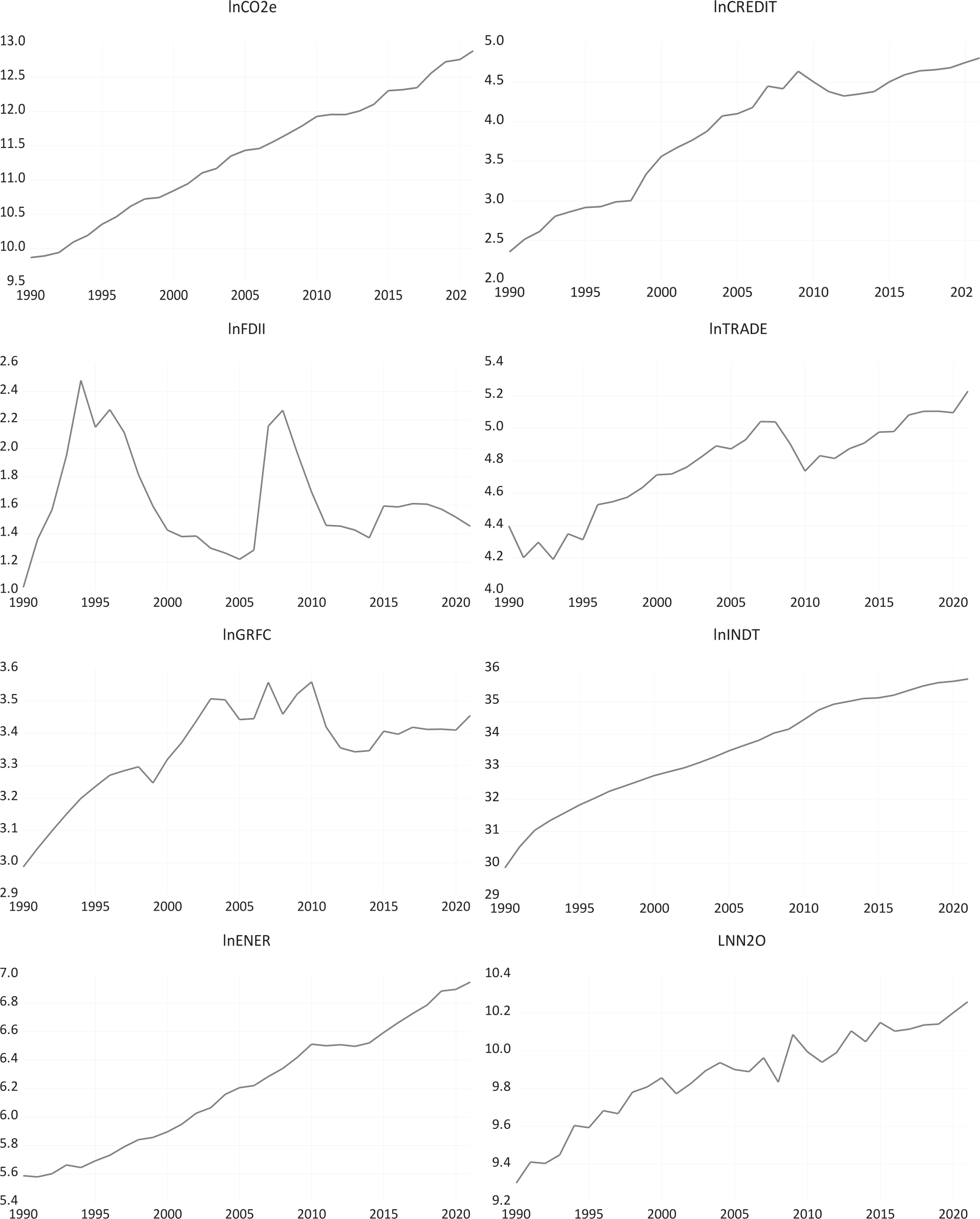
Fig. 1 shows the trends of all the variables to understand their movement over time. Specifically, the trend patterns of N2Oe, CREDIT, FDII, TRADE, and GRCF display a nonlinear pattern, whereas CO2e, INDT, and ENER increase periodically. A graphical assessment of the variables is insufficient to determine the nature of the relationships between them. Therefore, a critical analysis is essential.
Findings, Discussions, and Diagnostic Tests
Table 2 provides the descriptive statistics for all the variables. The median values were close to the mean values for most of the variables, indicating a symmetrical distribution. However, CO2e had a higher median (0.114) than the mean (0.054), showing a slightly positive skewness. The range of the data is highlighted by the maximum and minimum values, with CO2e having the widest range (−1.242 to 1.408) and GRFC the narrowest (2.987 to 3.560). The standard deviation, which measures the data dispersion from the mean, revealed that INDT had the highest standard deviation (1.637), making it the most volatile variable, whereas GRFC had the lowest (0.143), indicating that it was the least volatile.
Table 2.
Descriptive statistics.
Table 3.
Results of the stationary test.
Most variables exhibited negative skewness, indicating a slight left tail, except for FDII and ENER, which showed positive skewness, indicating a slight right tail. Kurtosis values close to three suggest a mesokurtic distribution (neither too peaked nor too flat), with GRFC having the highest kurtosis (3.235), indicating a slightly leptokurtic distribution. All variables had probability values greater than 0.05, suggesting that the null hypothesis of normality could not be rejected at the 5% significance level and that the variables were approximately normally distributed.
Table 3 presents the unit root test results for the stationarity of the variables. The unit roots of variables such as CO2e, N2Oe, CREDIT, TRADE, and ENER are at the level but stationary in their first differences, whereas FDII is stationary at the level. GRCF is stationary at the level in the ADF and PP tests, whereas the stationarity of this variable is found to differ when using the KPSS test. INDT shows stationarity at the difference level when employing the ADF test while considering the PP and KPSS test results. The unit root of INDT is stationary at this level. This suggests that the series in this study is a mixture of I(0) and I(1). The ARDL cointegration method is suitable for evaluating the long-term connection between variables, as per the unit root test results.
When selecting the lag length for empirical analysis, it is essential to choose appropriately. Inaccurate selection can affect the empirical results. We used the AIC, SC, FPE, and HQ criteria to determine the lag length. Given the small sample size of 32 observations, we started with a minimum of one lag order and gradually increased it to two to avoid over-parameterization. Table 4 displays the AIC, SC, and HQ results along with those of other tests to select lags based on the VAR model. Our model requires lag one as an appropriate setting, with CO2 and N2O serving as the dependent variables.
After determining the appropriate lag length, we applied the ARDL bounds test to analyze the long-term relationship between the variables, following the approach in [82]. Pesaran’s critical values are unsuitable for small sample sizes; therefore, [83] redefined them for the ARDL bound-testing approach to accommodate such sizes. Table 5 presents the findings of the ARDL bound-testing method for cointegration. The empirical results indicate long-term cointegration at the 5% significance level, as the calculated F-statistic exceeds the upper critical limit of 1%. This demonstrates the co-integration relationship between CO2 emissions and their determinants in the Vietnamese economy from 1990 to 2021.
Table 4.
Lag length criteria.
Table 5.
Bound test results.
Table 6 displays the dynamic models from the ARDL simulations of greenhouse gases over the long term. In Table 7, the error correction terms in all three regressions are significant and negative, indicating a long-term relationship between financial development, other emissions drivers, and environmental degradation. These findings are consistent with those of the cointegration tests. The significant coefficients of ECTt-1, −0.711 for CO2e, and −0.860 for N2Oe suggest that 71.1% of the CO2e and 86% of the N2Oe deviations from the long-term equilibrium are corrected each year.
As reported in Table 6, the coefficient of financial development (lnCREDIT) is negative and statistically significant, whereas the coefficient of the squared term (lnCREDIT2) is positive and significant. A 1% increase in lnCREDIT raises CO2e by 1.448% and N2Oe by 0.722%, respectively. Similarly, a 1% increase in lnCREDIT2 increases CO2 by 0.189% and N2O by 0.076%, respectively, indicating a U-shaped relationship. This suggests that financial development initially improves environmental quality, but later degrades it, which contradicts the EKC hypothesis for Vietnam and aligns with the findings of previous studies [47, 42]. However, Table 7 shows no statistical evidence of a U-shaped link between financial development and CO2e, whereas a significant U-shaped link between financial development and N2Oe is found in the short term. These findings indicate that the EKC hypothesis (inverted U-shaped link) is not confirmed in either the long or the short term. Interestingly, CO2e can only be reduced with an increase in financial development in the long term, whereas a reduction in N2Oe can be achieved before reaching a certain threshold for financial development in both the short and long term. This implies that the effects of financial development on CO2 emissions, such as increased energy consumption and industrial activity, take time to materialize and are more evident in the long term. Meanwhile, the financial sector growth has a more immediate and pronounced impact on N2O emissions. Thus, these results emphasise the importance of crafting financial policies that incentivise environmentally friendly investments, such as promoting green finance, to mitigate potential negative environmental impacts as the financial sector grows. The policies must focus on promoting financial growth, while ensuring environmental sustainability through stricter regulations for industries that contribute to higher emissions.
Table 6 shows the negative correlations between FDI and CO2 and N2O emissions. Specifically, a 1% increase in FDII reduces CO2e by 0.090% and N2Oe by 0.036%, respectively, holding other variables constant. This finding invalidates the PHH in Vietnam, aligns with [65] and [64], and contrasts with studies [62] and [63]. This study reveals that continuous FDI growth does not significantly contribute to environmental deterioration in Vietnam. Instead, it suggests that FDI improves environmental quality by fostering high-tech industry development. In the short term, the impact of FDII on CO2e was not statistically significant, but it significantly reduced N2Oe (see Table 7). Overall, FDI positively impacts environmental quality by reducing greenhouse gas emissions in both the short and long term. Our results challenge the PHH and suggest that foreign investments in Vietnam are fostering the development of cleaner high-tech industries. This confirms that facilitating the entry of environmentally conscious foreign investors could further strengthen Vietnam’s green economy and attract more FDI in sectors aligned with sustainable development goals (SDGs), thereby reinforcing the use of technology and innovation to improve environmental performance.
The empirical results in Tables 6–7 also show that trade openness negatively impacts Vietnam’s long- and short-term environmental quality. A 1% increase in TRADE decreased the environmental quality by 0.292% in terms of CO2e, although this effect was not observed for N2Oe. This supports the scale effect, in which increased trade leads to higher energy production and emissions. Developing countries may become “pollution havens” for industries moving from nations with stricter regulations, as supported by [68]. The insignificant impact on N2Oe indicates that trade openness does not uniformly affect all pollutants, with N2O produced mainly by agricultural rather than industrial activities. The environmental impact of trade openness depends on the trade sector composition; growth in less-polluting sectors may have a less harmful effect [69]. In the short term, TRADE significantly increased CO2e but not N2Oe. This suggests that increased trade leads to an immediate increase in carbon emissions owing to the expansion of export-oriented industries that rely on fossil fuels. However, the lack of a short-term impact on N2O emissions implies that the agricultural sector, which is primarily responsible for N2O emissions, is less responsive to short-term trade changes. Thus, incentivizing sustainable trade practices and fostering a transition towards less carbon-intensive industries could help mitigate the environmental impacts of increased trade. Trade practices that promote clean industries, particularly export-oriented sectors, should focus on reducing the negative impact of trading activities.
The coefficients of GRCF were statistically significant at 0.627 for CO2e and 0.834 for N2Oe, indicating that a 1% increase in GRCF raises CO2 emissions by 0.627% and N2O emissions by 0.834%, respectively. According to [84], careful environmental monitoring during capital formation can improve living standards without harming the environment (see Table 6). In the short term, the GRCF also positively and significantly affects both pollutants. A 1% increase in GRCF increases CO2e by 0.443% and N2Oe by 0.856%, respectively (see Table 7). This suggests that capital formation often compromises environmental quality, particularly in developing countries. Energy consumption and emissions increase as investment flows into infrastructure and manufacturing [85]. Overall, gross capital formation negatively impacts Vietnam’s environmental quality in both the short and long term, supporting the findings of [74]. Thus, investment in green infrastructure and cleaner technologies should be prioritized to ensure that economic growth does not occur at the cost of environmental degradation. This can be achieved by embedding environmental impact assessments and sustainable development requirements in the planning and execution of large-scale capital projects.
Moreover, a 1% increase in ENER leads to a 0.939% increase in CO2e, likely due to fossil fuel combustion, whereas there is no significant impact of energy consumption on N2Oe, as N2Oe is mainly associated with agricultural activities, such as fertilizer use and livestock production, and not energy use. This suggests that agricultural practices are the primary driver of N2O emissions in Vietnam. In the short term, ENER significantly increases CO2e but decreases N2Oe. This might be because energy consumption in the short term is directed towards sectors with lower N2O emissions, such as industry or transport, reducing overall N2O levels [79, 80]. INDT has a long-term negative impact on environmental quality in Vietnam. A 1% increase in industrial activity raises CO2 emissions by 0.22% and N2O emissions by 0.187% owing to increased energy use, particularly coal [86, 78]. However, the short-term results showed a significant negative relationship between INDT and CO2e, whereas no significant impact on N2Oe was reported. This may be because short-term industrial growth is skewed towards less carbon-intensive sectors, such as high-tech manufacturing or services, leading to an overall reduction in CO2 emissions. The lack of a significant relationship with N2O emissions was due to the different sources of N2O, primarily agricultural activities and land-use changes, compared to CO2 emissions. Emerging issues call for urgent action in Vietnam’s energy policies, such as toward renewable energy sources, reducing reliance on fossil fuels, and adopting sustainable farming techniques, which can play a crucial role in emissions reduction.
Table 6.
Long-run estimates for CO2e and N2Oe as dependent variables.
Table 7.
Short-run estimates for CO2e and N2Oe specifications.
Table 8.
Diagnostics test.
Additional diagnostic tests were performed to assess the statistical significance and reliability of the models. The results shown in Table 8 indicate no bias in the estimated results, confirming the reliability of the models. The p-values for the LM statistics of the CO2e and N2Oe equations were 0.195 and 0.164, respectively, and both were insignificant at the 5% level, indicating no serial correlation issues. The Jarque-Bera test showed that the residuals were normally distributed, and the Breusch-Pagan-Godfrey test indicated that the variance in the errors was constant, showing no heteroscedasticity. The Ramsay RESET tests for the CO2e and N2Oe equations had p-values of 0.7491 and 0.6853, respectively, confirming that the models were correctly specified.
Fig. 2.
Plot of CUSUM test and CUSUM of squared test. a) For CO2e equation, b) For N2Oe equation (Source: authors)
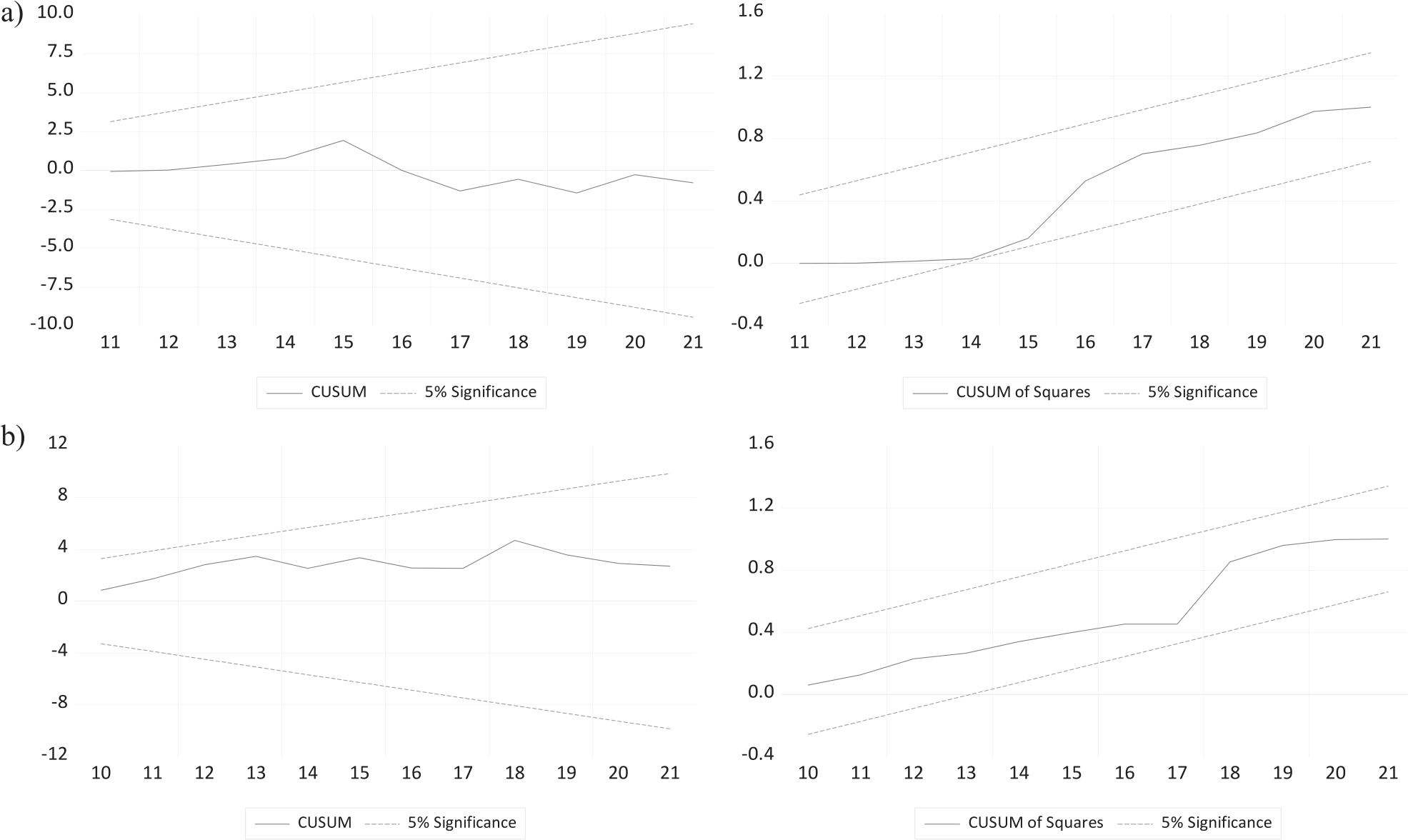
The following figures display two straight solid lines representing the 5% critical limit with a single dotted line between them. If the dotted line remained within the two solid lines, the null hypothesis regarding the validity of each estimated variable coefficient was accepted. However, the null hypothesis was rejected if the dotted line crossed the solid line and did not revert to the center. These results suggest that all estimated coefficients in the regression equations are dynamically stable (see Fig. 2).
Conclusion
This study investigates the relationship between financial development and environmental degradation in Vietnam by considering the potential existence of an EKC in terms of financial development. This study employs CO2 and N2O emissions as dependent variables and incorporates FDI, trade openness, gross capital formation, energy consumption, and industrial development as independent variables for annual data from 1990 to 2021. The ARDL approach was used to examine both long- and short-term dynamics, and diagnostic tests confirmed the robustness of the results. The main findings revealed a U-shaped relationship between financial development and emissions. Financial development initially improves environmental quality; however, later stages lead to deterioration. Specifically, FDI reduced both CO2 and N2O emissions, whereas trade openness negatively affected CO2 emissions in the long term. Gross capital formation and industrial development increased both CO2 and N2O emissions, and energy consumption significantly increased CO2 emissions but did not affect N2O emissions. In the short term, the U-shaped link between financial development and N2O emissions was significant but not for CO2 emissions. Trade openness positively affects CO2 emissions in the short term, whereas N2O emissions remain unaffected. All the regressions’ significant and negative error correction terms imply a long-term relationship among the variables.
Based on the empirical results, we suggest the following policy directions. First, the different short-term dynamics between financial development and CO2 and N2O emissions highlight the importance of considering the specific characteristics and response times of different greenhouse gases when examining the environmental impacts of the financial sector’s growth. Although the effects on CO2 emissions may be more gradual and long-term, their influence on N2O emissions appears to be more immediate and closely related to agricultural activities. Understanding these relationships is crucial for developing effective policies that can leverage the financial sector to mitigate CO2 and N2O emissions in Vietnam. Second, Vietnamese policymakers should adopt a proactive and balanced approach to address the U-shaped relationship between financial development and emissions. Encouraging green financing through incentives for clean energy investments and eco-friendly technologies is crucial during the early stages of financial development. As financial development progresses, stricter environmental regulations and emission standards must be implemented to curb potential ecological degradation. Third, attracting FDI in clean, high-tech industries can help leverage the technical impact of foreign investment based on the pollution halo hypothesis, while potentially minimizing its scale impact on emissions. Fourth, implementing stricter environmental regulations and emission standards for trade-oriented industries is crucial to counter the potential “pollution haven” effect and ensure that increased trade openness does not lead to environmental degradation. Fifth, environmentally responsible capital formation should be encouraged by integrating sustainability criteria into investment decisions and by promoting the adoption of clean technologies in the infrastructure and manufacturing sectors. Sixth, promoting energy efficiency and the transition to cleaner energy sources can help decouple economic growth from carbon emissions while also addressing the distinct drivers of N2O emissions in the agricultural sector. Finally, fostering the development of low-carbon high-tech industries is essential to ensure that industrial growth does not occur at the expense of environmental quality, particularly in the short term. By adopting this multifaceted approach, Vietnam can work towards sustainable development that balances economic growth with environmental protection.
This study has some limitations that suggest avenues for future research. First, focusing on a single country may limit the generalizability of our findings to other emerging markets. Future studies could extend this analysis to a panel of countries with similar economic conditions. Second, while CO2 and N2O are important greenhouse gases, incorporating other pollutants, such as CH4 and CFCs, could provide a more comprehensive view of the environmental impact. Third, additional variables, such as urbanization, institutional quality, and green technology adoption, could offer deeper insights into the complex interactions between economic growth, financial development, and environmental sustainability. By addressing these limitations, future research can build on the findings of this study and contribute to a more robust understanding of the environmental implications of financial development in emerging markets. This will inform the design of policies and strategies that promote sustainable economic growth while mitigating negative environmental consequences.

