

Introduction
Global warming, climate anomalies, and environmental pollution caused by carbon emissions are seriously threatening people’s health and sustainable economic development [1, 2]. In 2012, more than 3.7 million people died from air pollution, 88% of them in developing countries [3]. In the context of the global economic downturn, developing a low-carbon economy and achieving carbon decoupling has become an important international issue [4–7]. In 2016, nearly 200 parties around the world signed the Paris Agreement at the Paris Climate Change Conference. They are striving to meet the goal of keeping the rise in average global temperatures below 2°C above pre-industrial levels [8]. As a signatory to the Paris Agreement and the world’s largest carbon emitter, China has made a commitment to the world to achieve a carbon peak by 2030 and carbon neutrality by 2060, known as the “dual carbon” goal. It can be seen that China has placed a key position on developing a green economy and achieving a low-carbon transition.
There are many indicators to measure the low-carbon transition. Carbon productivity (CP) can be a bridge between economic output growth and low-carbon development, and has both economic output and carbon emissions, so it is often anchored as the expected target to balance the relationship between economic growth and carbon emission reduction. CP, first proposed by Kaya & Yokobori (1997) [9], refers to the ratio of gross domestic product (GDP) to carbon dioxide emissions in the same period. CP is used to measure the economic benefits created by unit carbon emissions [10, 11]. Currently, CP has been used by the Chinese government as an official indicator to measure how well provinces measure low-carbon transition [12–14]. According to the World Bank, China’s CP in 2020 was about $1,426 per ton, far below the global average of $1,635 per ton [15]. There is still a long way to go to improve the quality and efficiency of China’s CP. China still needs to take effective and feasible measures to improve CP. This is not only an important measure to accelerate the decoupling of economic growth from carbon, but also a powerful driver to promote low-carbon transformation of the economy and society.
According to the measurement definition of CP, the effective path to improve CP mainly focuses on two dimensions: promoting economic growth and promoting carbon emission reduction. From the perspective of economic development, Romer’s (1989) [16] endogenous growth theory believes that STI is the key factor in promoting long-term economic growth. The meeting of the Political Bureau of the CPC Central Committee clearly emphasized that STI is the primary driving force for China’s economic development, and STI should be regarded as the key factor to promote the high-quality development of China’s economy [17]. STI creates new production functions and introduces unprecedented new elements and conditions into the production system [18]. It can save production cost, improve production efficiency, promote the increase of output value and promote economic development [19]. From the perspective of carbon emission reduction, reasonable resource allocation is the cornerstone of production. STI can improve the energy consumption structure. Advanced technology can help companies make full use of renewable energy, such as solar and wind. Replace inefficient and highly polluting traditional biomass energy with clean energy to reduce energy costs and improve output efficiency. STI achieves carbon emission reduction through efficient energy allocation [20]. At the same time, the revolutionary breakthrough of technology is the catalyst for the development of Chinese-style new quality productivity [21]. The new quality productivity promoted by STI can enrich the expression form of social production tools, promote the intelligence of the industrial production process, improve the efficiency of resource utilization and resource sharing, realize cleaner and green production, and achieve the purpose of carbon emission reduction. In conclusion, STI can promote both economic growth and carbon emission reduction. Therefore, it can be regarded as the fundamental path to improve CP. At present, studies on the relationship between STI and economic development or the relationship between STI and carbon emissions are relatively common in academia. However, studies that directly focus on the relationship between STI and CP are still few and need to be further explored. To explore the above issues, this study first explored the direct link between STI and CP using the two-way fixed effects model as the benchmark model. Subsequently, the spatial spillover effect of STI on CP is explored through the spatial Durbin model, and the regional heterogeneity of this spillover effect is analyzed. Finally, we further discuss the threshold effect of STI on CP based on STI and R&D intensity. The rest of this paper is arranged as follows: Section 2 reviews the relevant literature. Section 3 presents the research methodology. Section 4 presents the empirical results. Section 5 provides a further discussion of the findings. Section 6 summarizes the findings and provides policy recommendations.
Literature Review
Although CP and STI are both hot topics in current academic research, there is still little literature on the direct relationship between the two.
This study will review the research status of the two in their respective fields. The current academic research on CP mainly focuses on two aspects: measurement methods and influencing factors. Since Kaya & Yokobori [9] proposed the ratio of gross domestic product to carbon dioxide emissions in the same period as the measurement method of CP, a variety of measurement standards of CP have been derived on this basis. However, studies focusing on the relationship between economic development and CP still often use the measurement index proposed by Kaya & Yokobori [9] to evaluate CP. This paper aims to explore the low-carbon economic path of economic development and carbon emission reduction through STI, so this classical measurement method is also selected. Other methods include the Malmquist index calculated based on the DEA proposed by Fare et al. [22]. The Malmquist-Luenberger (ML) index, which incorporates unexpected output into the Malmquist index, is a more comprehensive measurement method. These methods take into account the relationship between energy, human, capital, and carbon emission reduction. It is mostly used in articles studying the relationship between total factor production efficiency and carbon emissions [23, 24]. The research on the influencing factors of CP mainly focuses on environmental policy, R&D investment, industrial structure transformation, and other aspects. Zhao et al. [25] found that environmentally induced R&D investment can effectively improve CP. The investment will produce a positive spatial spillover effect while improving CP. This also has a positive impact on adjacent areas. The study of Sheng et al. [26] further confirms the above views. Zhang [27] found that low-carbon city pilot policies can improve CP, and the local and neighboring impacts of environmental regulation on CP show U-shaped characteristics. In addition, Niu et al. [28] also emphasized the impact of economic activities and industrial structure on regional CP.
Most of the research on STI focuses on two perspectives: influencing factors and effects [29–31]. From the perspective of the influencing factors of STI, Song et al. [32] found that the digital economy was an important boost to STI development. It can improve the STI level from multiple perspectives of quantity and quality. At the same time, the utility of the digital economy also has a significant spatial spillover effect [33]. Li et al. [34] explored the U-shaped nonlinear relationship between corporate environmental responsibility and green STI from the perspective of enterprises. At the same time, STI will also be affected by the level of ESG disclosure and corporate financing constraints [35]. The closeness of the relationship between the firm and the bank will also have utility on STI [36]. Research on the effect role of STI has mainly focused on the field of energy use. Li et al. [37] confirmed that STI can reduce the negative economic benefits brought by resource extraction and promote sustainable economic development. Xu et al. [38] also found that STI of clean energy can improve energy efficiency. Acheampong et al. [39] also pointed out that STI can promote low-carbon economic development from multiple dimensions of energy transition, environmental governance, and economic growth. At the same time, some scholars have discussed the relationship between STI and total factor CP in the energy field. Li et al. [40] found that innovation in renewable energy technology can promote the improvement of green total factor productivity. To sum up, the research on STI in energy utilization, production efficiency, and other fields has gradually become mature. This provides part of the basis for us to infer that STI achieves carbon emission reduction and economic development by improving energy efficiency. However, there is still less work on the relationship between STI and CP. Based on this, this paper will conduct in-depth research on this topic from the perspective of spatial spillover and threshold effect.
Materials and Methods
Model Elaboration
Bidirectional Fixed-Effect Model of Baseline Regression
First, based on the overall impact of STI on CP, a benchmark regression model is constructed:
Where, the subscript i represents the 30 provinces in the sample data, and t represents the specific years from 2011 to 2021. CP represents carbon productivity and STI represents the scientific and technological innovation level. Represents the control variable, rt is the time-fixed effect, ui is the region-fixed effect, εi,t represents the random disturbance term.
Spatial Econometric Model
Spatial Autocorrelation Test
The necessary condition for considering the existence of spatial effect is the existence of spatial autocorrelation. Spatial autocorrelation refers to the potential interdependence of some variables within the same distribution area of observational data. It is a measure of the degree of clustering of spatial unit attribute values. In order to describe the overall spatial relationship among units in the study area, this study uses the global Moran’s I index to measure the spatial correlation of STI in 30 provinces in China during 2011–2021. The specific calculation formula is constructed as follows:
Where, N is the number of provinces, xi, and xj represent the level of technological innovation and carbon productivity of each province, and W represents the spatial weight value.
Construct the Spatial Durbin Model
In order to explore the spatial spillover effect of STI on CP, after a series of tests on the effectiveness of the spatial econometric model, this paper finally adopts the spatial Durbin model (SDM) to study the above problems. The specific calculation formula is constructed as follows:
Where W represents the spatial weight matrix, α1, βj represent the direct effects of STI and other control variables respectively. ρ, ψ1, and ξ represent the spatial spillover effects of CP, STI, and other control variables, respectively. The remaining variables and symbols have the same meaning as (1).
Decomposition of Direct and Indirect Effects
In the spatial Durbin model, the independent variable coefficients estimated by SDM include the spatial spillover effect of neighboring regions and the influence of local provinces on neighboring provinces. Therefore, the SDM coefficient cannot accurately estimate the marginal effect of an independent variable on a dependent variable. With reference to Weng et al (2023) [41], we rewrite the equation.
Where, Yt represents the dependent variable. Xt represents the independent variable. Rt represents the residual term of the intercept term and the error term.
For the KTH independent variable from unit 1 to unit N, the expected value of the partial derivative matrix Yt can be written as the following equation.
Here, we assume that the KTH independent variable is STI and the dependent variable is CP. When i=j, the corresponding element in the partial derivative matrix lies on the principal diagonal. In this case, it represents the CP factor assessment of the change in STI in that province to that province. This reflects the direct impact of the province. When i≠j, the corresponding element in the partial derivative matrix lies on a non-diagonal line. In this case, it represents the indirect influencing factor between neighboring provinces and reflects the influence of provincial STI changes on CP in neighboring provinces. Such indirect effects are also known as spillovers. The sum of direct and indirect effects is the total effect.
Select the Space Matrix
Considering that the regression results are sensitive to the selection of spatial weights, this paper uses a variety of spatial weight matrices to perform spatial econometric regression.
1. Spatial adjacency matrix: Considering that the adjacency relationship between regions is an important factor affecting the spatial effect, the spatial adjacency matrix is constructed. If the two cities are adjacent, the value is 1, otherwise it is 0.
2. Economic geography nested matrix: The economic relations between regions will also affect the spatial effect. In order to comprehensively investigate the dual influence of economic and geographical factors, the nested matrix of economic distance and geographical distance weight matrix is further used as the base measurement matrix. Is the square of the geographical distance between provinces i and j.
3. This paper adopts a geographic nested matrix based on latitude and longitude to conduct a robustness test, representing the square number of latitude and longitude distances of provinces i and j.
Threshold Effect Model
In order to further examine and verify the nonlinear relationship between STI and carbon productivity, we proposed a threshold regression model based on Hansen (1999) [42]. The model is as follows:
In the above formula, STI and RD in parentheses are threshold variables. r is the threshold to be estimated. I (·) is the indicator function. If the condition is met, the value is 1; otherwise, the value is 0. The meaning of the remaining variables and symbols is exactly the same as (1).
Measurement of Variable
Explained Variable
Considering that CP should reflect both the level of carbon emissions and economic development, this paper refers to the measurement method of CP proposed by Kaya & Yokobori (1997) [9] and the official standard of Chinese government departments [12]. CP is measured by calculating the economic output value per unit of carbon dioxide emissions. The specific formula is as follows:
Where CO2 represents the total carbon dioxide emissions. It is measured by combining the research of Sun et al., (2023) [43]. Represents the type of energy, including the carbon emissions of eight energy sources: raw coal, coke, crude oil, gasoline, kerosene, diesel, fuel oil, and natural gas. Ei represents total energy consumption. NCVi, CCi, and COFi represent the average low calorific value, carbon content, and carbonization coefficient of each type of energy, respectively. 44 and 12 represent the molecular weights of carbon dioxide and carbon, respectively. CP can be obtained by dividing the GDP by the calculated CO2.
Explanatory Variable
Due to the easy availability and accuracy of the number of patents, it is generally used as an indicator to measure technological innovation [44, 45]. On the basis of related research, this paper takes the number of invention patents accepted as an index to measure technological innovation.
Referring to [43, 47], taking into account other factors affecting CP, in this paper, indicators such as environmental tax revenue and industrialization level are used as control variables. At the same time, in order to further explore the threshold effect of STI on CP, this study sets the level of technological innovation, the core explanatory variable, and R&D intensity in the control variable as the threshold variable.
Data Source
All the variable data in this paper come from authoritative yearbooks such as China Statistical Yearbook, China Statistical Yearbook on Energy, China Statistical Yearbook on Science and Technology, China Statistical Yearbook on Industry, Ministry of Finance, PRC, and China Population and Employment Statistical Yearbook [48–53]. The data type is the panel data of 30 Chinese provinces (excluding Taiwan, Hong Kong, Macao, and Tibet) from 2011 to 2021. The specific variables and descriptive statistics are shown in Tables 2 and 3.
Results and Discussion
Analysis of Temporal and Spatial Characteristics of Carbon Productivity
This study measured the carbon productivity of 30 provinces in China from 2011 to 2021 by formulas (1) and (2), and used stata17.0 software to visualize the carbon productivity of 30 provinces in 2011, 2014, 2017, and 2021 in time and space. Details are shown in Fig. 1.
Analysis of longitudinal time trends from 2011 to 2021 shows that China’s carbon productivity as a whole has shown a steady upward trend. In 2011, most provinces showed a low level of CP and a lighter color. As time goes on, especially in 2017 and 2021, it is clear that more provinces will turn darker. In the economically developed east coast and other places, this upward trend is particularly obvious. We speculate that this is closely related to the progress of technological innovation in various regions, the optimization and upgrading of the industrial structure, and the low-carbon economic policies of government departments.
From the analysis of horizontal regional differences, there are significant differences in CP levels between the eastern and western provinces, especially between the eastern coastal and inland provinces. The CP of the eastern coastal areas is generally higher than that of the inland provinces, and the color tends to be more red. Based on this, we speculate that this may reflect more advanced science and technology and more efficient resource utilization in these areas. In contrast, the CP of western regions, such as Gansu and Qinghai, is not only low in general, but also grows slowly, which reflects that the inland regions in northwest China are still facing severe challenges in carbon decoupling. The overall level of CP in southern provinces, such as Guangdong, is extremely high and growing rapidly. However, the CP level of northern provinces, such as Heilongjiang and Jilin, obviously shows the problem of lagging development. This may be due to the cold climate in northeast China, which requires the consumption of a large amount of biomass energy with high energy consumption to obtain heat in winter, resulting in high carbon emissions. At the same time, the economic foundation of northeast China is weak and the momentum of economic development is insufficient. The influence of the above double factors eventually leads to the weak state of CP.
Table 1.
Variables and measurement methods.
Table 2.
Descriptive statistics.
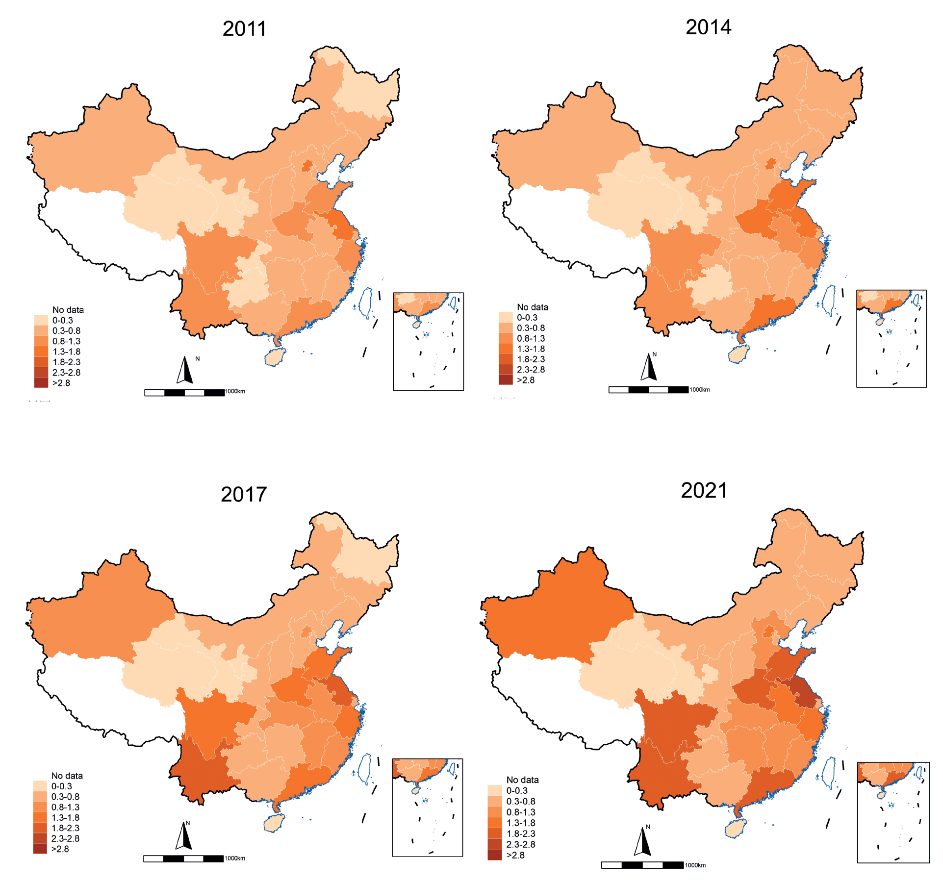
To sum up, China’s CP shows the characteristics of spatial and temporal differentiation with generally stable growth and significant inter-regional differences. On the one hand, it reflects the active efforts of the state in environmental governance and sustainable economic development. On the other hand, it also shows that there is still a certain degree of regional incoordination in the development of the low-carbon economy among Chinese provinces.
Multicollinearity Test and Hausman Test
In order to avoid the correlation between explanatory variables and multiple control variables affecting subsequent results, the model needs to be tested for multicollinearity. This paper uses the variance inflation factor (VIF) to conduct a multicollinearity test. The test results show that the VIF value of each variable is less than 10, and the mean VIF is 3.7, indicating that there is no multicollinearity in the model. Therefore, the selected variables can be used in the model analysis.
In this paper, the Hausman test is used to select a more efficient estimation model. The details are shown in Table 3. Table 3 shows that the p-value of the Hausman test is 0.000. This shows that the hypothesis of the random effect model is rejected at the significance level of 0.01, so the fixed effect model should be used.
Benchmark Regression Results
To explore the impact of STI on CP, we used the two-way fixed effects model as the benchmark model for regression. In order to ensure the reliability of the regression results, we also show the regression results of the OLS and RE models. The details are shown in Table 4. Among them, models (1), (3), and (5) are regression results without adding the threshold variable RD. (2), (4), and (6) are regression results with RD taken into account. It can be seen that in the regression of the fixed effect model, the coefficient of STI is positive and passes the significance test at least at the 5% level. Taking Column (4) of Table 4 as an example, the economic significance of the STI coefficient is expressed as that for every 1% increase in STI, CP will increase by about 0.096%. This indicates that STI has a significant positive effect on CP from a national perspective. By improving STI, cleaner and more efficient technologies can be applied to production, energy consumption structure can be improved, energy utilization efficiency can be improved, industrial transformation and upgrading can be promoted to a green and low-carbon direction, and high-quality low-carbon economy can be developed, so as to improve CP level.
Robustness and Endogeneity Test of Benchmark Model
Robustness Test
In order to ensure the stability and reliability of the benchmark regression results, we successively add control variables. We use the stepwise regression method to test the model’s robustness. The detailed results are shown in columns (1)–(4) of Table 5. In the process of gradually adding control variables, the core explanatory variable STI always has a significantly positive correlation with the explained variable CP. This shows that the estimation results of the final model are reliable.
At the same time, we also use the method of replacing explanatory variables to further conduct robustness test. We put the core explanatory variable STI lagged by one period into the model for regression. The specific results are shown in Column (5) of Table 5. It can be seen from the results of Column (5) that the regression coefficient of the first-order lagged term of STI on CP is 0.074. And it is significant at the 5% level. This once again verifies the positive effect of STI on CP. The above conclusions prove the reliability of the underlying regression model.
Endogeneity Test
The SYS-GMM model is superior in dealing with the problem of endogenous variables. By selecting appropriate instrumental variables, the possible bias caused by endogenous explanatory variables can be effectively alleviated [54]. In this study, the first-order lag term of the explanatory variable STI and the first-order lag term of some control variables are selected as instrumental variables, and the SYS-GMM model is used for endogeneity test. As can be seen from Table 6, the Hansen overidentification test results show that the p-value is greater than 0.1, indicating that the selection of instrumental variables is effective. The p-value of AR (2) is greater than 0.1, indicating that the model does not have serial autocorrelation above the second order. Based on the above results, it is judged that the current SYS-GMM model is well constructed. At the same time, the coefficient of STI is significantly positive, which confirms that the endogeneity test of the model basically passes.
Table 4.
Benchmark regression results.
Regression of Spatial Econometric Model
Spatial Correlation Analysis of STI and CP
In this paper, the spatial distance weight matrix is used to calculate the Moran index I of STI and CP. The specific calculation results are shown in Table 7. It can be seen from Table 7 that both the Moran index of STI and CP passed the significance test. This indicates that both technological innovation and CP have significant spatial agglomeration characteristics. Among them, the Moran index of STI has a rising trend year by year. The spatial correlation of STI increased year by year. The Moran index of CP showed a fluctuating downward trend. It shows that the spatial autocorrelation decreases slightly year by year.
In order to clearly observe the spatial agglomeration characteristics of technological innovation and CP, this study draws the spatial scatterplot of technological innovation and CP in 2021.
Table 5.
Results of stepwise regressions and robustness tests.
As shown in Fig. 3. Among them, (1) is the spatial scatterplot of technological innovation. (2) is the spatial scatterplot of CP. It can be seen that the Molan index of STI and CP are mostly located in the first and third quadrants. This shows that the spatial correlation between the regions is high, with a high degree of agglomeration characteristics. Therefore, in the study of the relationship between the two should pay attention to the analysis of spatial factors.
Test of Spatial Metrology Model Selection
In order to select a more suitable spatial measurement model, LM, LR, Wald, and other tests were carried out in this study. The test results are shown in Table 8, and LM test results are significant at 1% and 5% levels. This suggests that a spatial effect model can be chosen. In addition, the results of both the Wald test and the LR test were significant at the 5% level. This indicates that the null hypothesis of selecting SRM and SEM models is negated. This means that both the spatial error term and the spatial lag term exist simultaneously. Therefore, this paper should choose the spatial Durbin model (SDM) which combines the two. At the same time, in the LR test to judge the selection of time-fixed effect, regional fixed effect, and two-way fixed effect, both the time-fixed effect and space-fixed effect are significant at the level of 1%. This represents a rejection of the respective null hypothesis. Therefore, the spatial Durbin model of bidirectional fixed effects is finally chosen.
Regression Results of Spatial Durbin Model
According to the results of spatial correlation analysis in 4.5.1, both STI and CP have strong spatial correlation. In order to further explore the spatial effect and spatial spillover effect of STI on CP, the spatial neighbor matrix and spatial economic geography matrix are selected in this section. In this paper, the spatial influence mechanism of STI on CP is discussed by using the spatial Durbin model. Table 9 shows the regression results of the spatial Durbin model.
It can be seen from the results in Table 9 that in the regression of spatial adjacency matrix and spatial economic and geographic nested matrix, the estimated coefficients of STI are significantly positive at the 1% confidence level. This indicates that the development of STI in this region contributes to the improvement of CP in this region. Specifically, take the regression results of the nested matrix of spatial economic geography as an example. A 1% increase in STI in a given area will promote a 0.09% increase in CP in that area. At the same time, the spatial lag coefficient of STI is significantly positive. This indicates that STI in the local area has positive externalities to neighboring areas. This can promote the improvement of CP in neighboring areas. It is worth noting that the spatial lag term coefficient of CP is significantly negative in the regression of both matrices. It shows that there is a significant negative spatial spillover effect of CP development in China. The regression results of the nested matrix of spatial economic geography are also taken as an example. A 1% increase in the CP level in the neighboring area resulted in a 0.351% decrease in the local CP level. This may be due to factors such as rapid economic growth and rapid improvement of production efficiency, which make the developed areas with high CP have a “siphon effect” on the surrounding areas to a certain extent. As a result, various factor resources such as talent, technology, and capital are concentrated in this region, thus inhibiting CP development in surrounding areas [55–57].
Because the spatial Durbin model contains the spatial lag term of the dependent variable, there is an error in the estimation coefficient. Based on this, this study uses partial differential matrix operation to divide the total effect of independent variables on dependent variables into direct effect and indirect effect [58]. Table 10 shows the decomposition estimation results of the spatial spillover effect.
Table 7.
Global Moran Index.
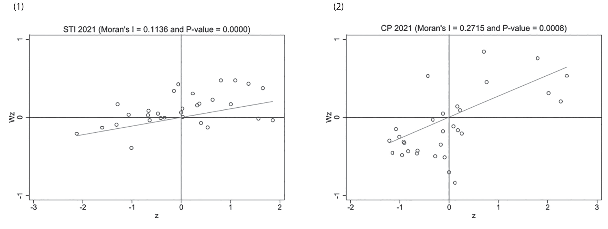
Table 8.
Spatial measurement model selection test.
As can be seen from Table 10, the direct effect of STI on regional CP growth is significantly positive. Specifically, take the regression results of the nested matrix of spatial economic geography as an example. When STI increases by 1% in a certain area, CP increases by 0.082%. The indirect effect is also significantly positive and larger than the direct effect. The results reveal the direct and spatial spillover effects of STI on CP. On the one hand, the progress of STI has a significant positive impact on the local CP, which is consistent with the regression results of the spatial Durbin model in Table 9. This is because STI can promote the improvement of local CP by improving the energy consumption structure, improving the efficiency of resource utilization, and developing advanced productivity. Clean, efficient, and advanced technologies help reduce carbon emissions in the production process and increase the added value of production, thereby improving CP. On the other hand, the indirect effect is significantly positive and larger than the direct effect. This indicates that the STI in the region not only promotes local CP improvement but also has a positive impact on the surrounding areas. Local STI can promote the improvement of CP levels in many surrounding areas. To some extent, this reflects the diffusion of innovation and the radiation effect of technology brought about by STI. Good technology in one region can be spread and diffused between regions. Each region improves its own CP by adopting and using advanced technologies from other regions [59]. The spatial spillover effect of STI helps to realize the coordinated development between regions, reduce the gap of CP development level between regions, and form a virtuous circle of sustainable development patterns of the low-carbon economy between regions.
Table 9.
Panel data regression results of the spatial Durbin model.
Based on this, while promoting STI, local governments should also pay attention to the development of inter-regional technology complementarity and technology radiation capabilities. Create a “thriving land” of scientific and technological innovation, and spread local scientific and technological achievements and high and new technologies to the outside world. Exchange needed goods, give play to the linkage effect of science and technology, and strengthen the chain function of various regions in the national innovation network.
Table 10.
Decomposition results of spatial spillover effects.
Robustness Test of Spatial Durbin Model
In order to ensure the accuracy of the estimation results, this paper uses the latitude and longitude distance matrix as the spatial weight matrix for the robustness test. Table 11 shows the results of the robustness test. It can be found that the influence coefficient of the core explanatory variable STI in Table 11 on the explained variable CP is significantly positive, which is basically consistent with the above results. At the same time, the direction and significance of the effect decomposition of other control variables are basically the same as those of the above variables, indicating that the estimation results in this paper are robust.
Regional Heterogeneity Analysis
According to the research results, the development of CP has the characteristics of spatial and temporal differentiation, and the level of CP varies significantly among regions. Therefore, this section will discuss the regional heterogeneity of technological innovation in CP from the perspectives of the eastern, central, and western regions of the country. Table 12 shows the results of the regional heterogeneity analysis based on the spatial Durbin model.
Based on the analysis of Table 12, it can be seen from the regression results of the spatial Durbin model that the technological innovation coefficient of the eastern region is significantly positive. However, the technological innovation coefficient of central and western regions is not significant. This indicates that the increase of STI has a significant positive effect on local CP in the eastern region, but not in the central and western regions. This may be due to the better STI foundation in the eastern region, strong innovation capacity, high innovation efficiency, and the easier process of transforming technological innovation into advanced productivity. Therefore, the eastern region can promote the development of CP through technological development [60, 61]. At the same time, the economic strength of the eastern region is strong, the financing of relevant innovative enterprises is relatively convenient, the cost of technological innovation is low, and the economic benefits brought by innovation are obvious. Therefore, technological innovation has a significant effect on improving CP [62, 63]. For the central and western regions, due to the weak local technical and economic foundation, high cost, and long cycle of technological innovation, the process of transforming into advanced productive forces is extremely difficult, and the economic benefit of growth brought by technological progress cannot even make up for the initial capital investment. As a result, the effect of STI on CP is not significant [64, 65].
Table 11.
Robustness test of spatial Durbin model.
According to the effect decomposition by partial differential method, the direct and indirect effects of STI on CP are still only positive in the eastern region. This indicates that STI in the eastern region has a positive effect on CP development in the local and neighboring areas. The eastern region is the gathering center of science and technology innovation in China, and the core STI capability is strong. STI can produce a linkage with CP development at the time and space level to achieve the effect of spillover divergence. At the same time, the eastern market economy is more developed, the flow speed of technology in the market is faster, and the market orientation is strong, which can play the role of market mechanism to effectively spread high-tech. Compared with the eastern region, the technological development of the central and western regions is still not mature enough, the quality of innovation needs to be improved, and more powerful STI and technological progress are needed [66, 67]. Therefore, it is necessary to continue to promote the “rise of the central region” work and implement the “western development” strategy. These measures promote regional coordinated development to achieve the technological maturity of the eastern region, which can be diffused to the central and western regions, and further enhance the ability of independent innovation in the central and western regions.
Table 12.
Regional heterogeneity analysis.
Threshold Effect Analysis
Threshold Effect Test
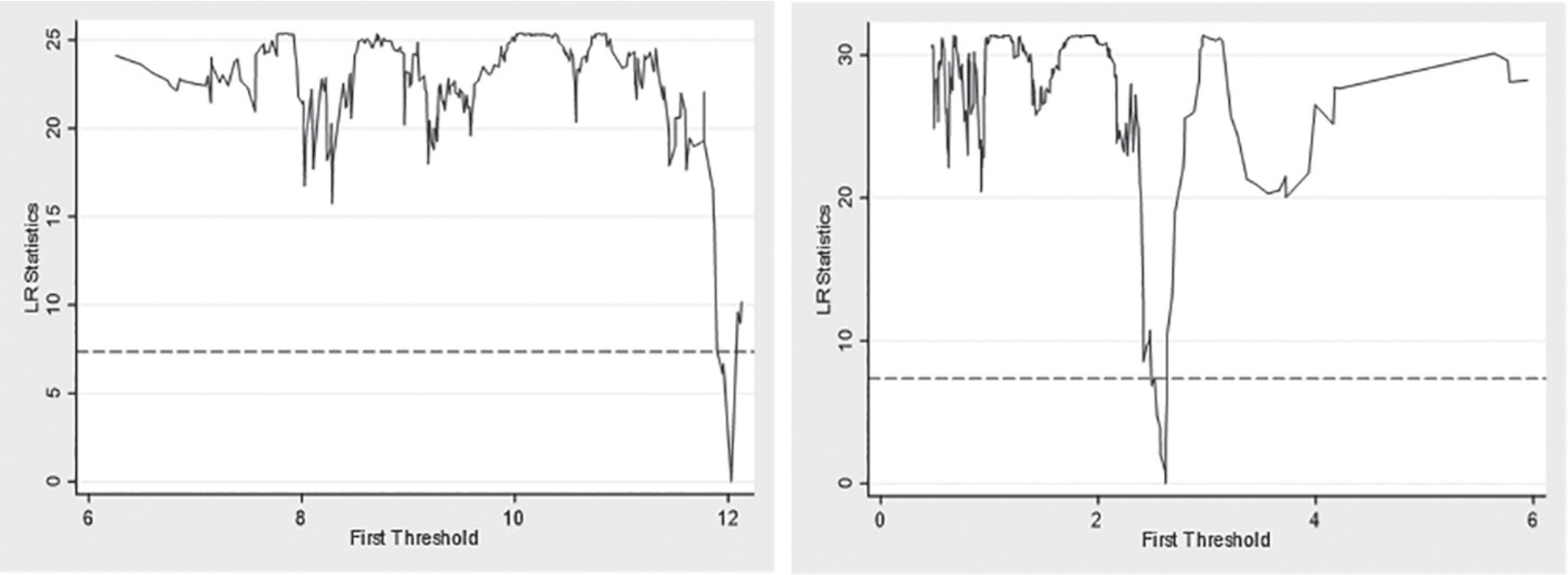
Relevant studies have found that STI has the characteristics of low return in the early stage, long cycle, high risk, etc., and its role often needs to reach a sufficient level to play [68, 69]. The regional heterogeneity test also confirmed that STI had a more significant positive effect on CP in the eastern region, with a better STI foundation and stronger financial support. Therefore, we speculate that the effect of STI on CP may be related to its own level of basic development and related research and development funding support. Therefore, this study takes STI and RD as threshold variables to discuss the nonlinear threshold effect of STI on CP. First, STI and RD were taken as threshold variables, respectively. The threshold effect test was conducted by using the Bootstrap method for 300 samples. The test results are shown in Table 13 and Fig. 3. It can be seen from the results of F-value and P-value that STI and RD as threshold variables pass the single threshold test at the level of 10%. Therefore, the influence of STI on CP has a single threshold effect of STI and research and development fund support. The threshold values are 12.029 and 2.618, respectively.
Regression Results and Analysis of Threshold Model
Table 14 shows the regression results of the threshold model. According to Column (1), STI has a nonlinear positive effect on CP. When the development level of STI crosses the threshold value of 12.029, the regression coefficient changes from 0.073 to 0.098, and the significance degree changes from the confidence level of 10% to the confidence level of 5%. This indicates that the promotion effect of STI on CP is enhanced in areas with a high STI base. It can be seen from Column (2) that when the R&D intensity is less than the threshold value of 2.618, every 1% increase in STI can increase CP by 0.072%; When the R&D intensity is greater than the threshold value, every 1% increase in STI can increase CP by 0.096%. This verifies that when the level of R&D investment and financial support is high, the positive utility of STI on CP will also be stronger. The above findings further explain the differential utility of STI to CP in different regions in the regional heterogeneity analysis.
Conclusions
Research Conclusions
This paper measures the level of technological innovation and CP in 30 provinces of China from 2011 to 2021 by introducing two measurement methods. The direct effect, spatial spillover effect, and threshold effect of STI on CP were also explored through a two-way fixed effect model, spatial Durbin model, and single threshold effect model. The study found that:
1. STI can not only promote the development of local CP, but also has a positive spatial spillover effect, which can drive the improvement of CP in surrounding areas. This conclusion is still valid after the robustness test.
2. There are regional differences in the effect of STI on CP. In the eastern region, STI has a significant positive utility for CP in local and neighboring provinces; In the central and western regions, these effects are not obvious.
3. Under the premise that STI and RD are threshold variables, there is a single threshold effect in the impact of STI on CP. Specifically, when STI exceeds the threshold value of 12.029, the influence coefficient of STI on CP increases from 0.073 to 0.098; When the R&D intensity exceeds the threshold value of 2.618, the influence coefficient of STI on CP increases from 0.072 to 0.096.
Policy Recommendations
Based on the above research results, we put forward the following policy suggestions to promote the improvement of CP and the development of a low-carbon economy:
1. Encouraging and stimulating STI in various regions through policy measures. STI is a strong driving force for developing a low-carbon economy and accelerat-ing the decoupling of economic growth from carbon emissions. We can provide a good agglomeration environment and infrastructure for STI-type enterprises through the construction of an innovation ecosystem and the development of innovation parks, so as to promote the improvement of STI.
2. Strengthening STI R&D and cooperation among regions. STI has a positive spatial spillover effect on the development of CP, and the cooperation and linkage among regions are key to maximizing the positive impact of STI. Government departments can promote technology sharing and cooperation among different regions by establishing inter-regional technology transfer platforms. Encouraging knowledge sharing and technology exchange can create a good mutually beneficial environment for the development of the low-carbon economy.
Table 15.
Threshold effect regression results.
| Explanatory variable | Threshold variable | |
|---|---|---|
| (1) | (2) | |
| STI | RD | |
| STI0 | 0.073* | 0.072* |
| (0.036) | (0.035) | |
| STI1 | 0.098** | 0.096** |
| (0.036) | (0.036) | |
| Control variable | YES | YES |
| AREA | YES | YES |
| YEAR | YES | YES |
| N | 330 | 330 |
| R-squared | 0.6248 | 0.6317 |
3. The paper will formulate targeted innovative development strategies based on regional differences. The role of STI varies significantly in different regions and at different stages of development, and relevant policies should be adjusted according to regional characteristics, technological base, and funding level. On the one hand, the policy can focus on expanding the existing STI benefits, optimizing the STI transmission path, and spreading the advanced technology to other regions. On the other hand, it can focus on exploring a new path for STI to promote the development of the low-carbon economy and improve the development of more advanced productivity with high-quality technology. In the central and western regions, where the foundation of technology development is weak and R&D funds are in short supply, it is necessary to increase financial support for local scientific research institu-tions and R&D enterprises, provide subsidiary-type STI financial policies, alleviate the problems of financing difficulties, poor facilities and high risks in technology R&D, and encourage innovative enterprises to increase R&D investment to improve basic STI.
Research Limitations and Future Prospects
At present, there is still room for further expansion of this study. Firstly, studies rely mainly on past statistics, which may fail to adequately capture the diversification factors affecting STI and CP. Secondly, due to the time and geographical scope limitations of the data, the conclusions of this paper may not be applicable to all countries or regions in the world. Finally, with the development of advanced spatial econometric methods, the spatial effects of STI on CP can be explored more accurately.

