

Introduction
Climate change caused by the continuous growth of greenhouse gas emissions has received widespread attention in past decades, posing significant threats to the global sustainability of human and economic development. Currently, there is a consensus within the international community to address climate change and reduce carbon emissions [1], as exemplified by the Paris Climate Accords, which were adopted by nearly 200 parties in 2015. These goals point to fostering a green economy that harmonizes both economic growth and the ecological environment and are argued to effectively promote the process of stabilizing growth and offering opportunities to create new jobs [2].
The low-carbon transformation of the real economy involves a coordinated deployment of financial resources, rendering financing one of the essential challenges throughout the transformation process, as highlighted by the United Nations Environment Programme (UNEP). The OECD estimates that approximately 7 trillion dollars per year will be required globally to meet the objectives outlined in the Paris Climate Accords by 2030. With such a substantial amount of financial resources needed, it is imperative to reorient both the public and private financial sectors to actively support sustainable investment and innovation. The importance of scaling up green finance has thus been recognized, leading to its inclusion as a vital topic for the first time on the G20 summit agenda in 2016.
Green finance refers to the financial services provided for economic activities that support environmental improvement, mitigate climate change, and utilize resources more efficiently. It has the dual characteristics of financial resource allocation and environmental regulation. The green financial system utilizes a series of financial instruments, including green credit, green bonds, green stocks, green development funds, green insurance, and carbon finance, to support the green transformation of the economy. In this context, green finance, guided by the goals of carbon peaking, carbon neutrality, and green development, will become an important direction for future financial development and construction around the world. For example, the European Commission set out a comprehensive EU strategy in its 2018 action plan on sustainable finance to strengthen the connection between finance and sustainability.
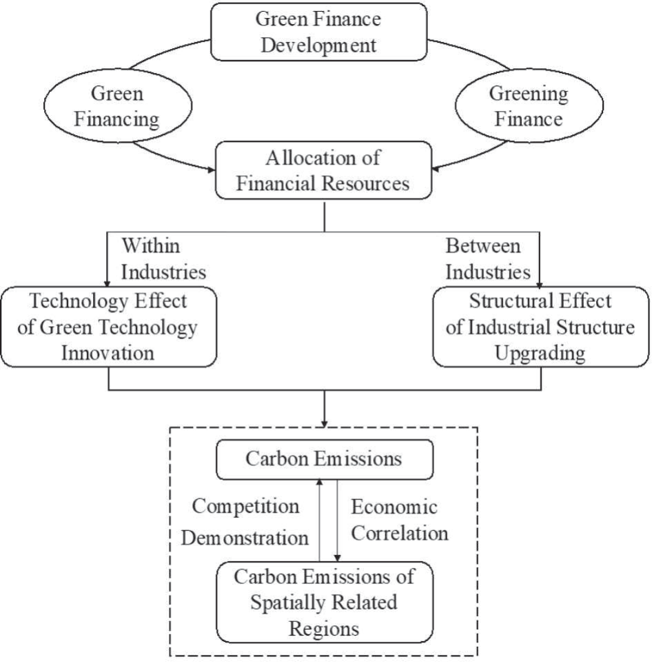
Note that green finance development and carbon emission reduction, as important driving forces and target functions of economic transformation and development, respectively, may have an inherent linkage that cannot be ignored. We hypothesize that green finance development influences carbon emissions through two mechanisms: the technology effect of green technology innovation (within industries) and the structural effect of industrial structure upgrading (between industries). On one hand, compared to the traditional financial system, green finance emphasizes that the financial sector needs to fully consider the potential benefits and risks associated with environmental conditions in the process of financial allocation decisions so as to promote long-term sustainable economic and social development [3]. Green finance development allows green enterprises more comparative advantages in receiving financial resources for further production and innovation and compels other enterprises in the same industry to embrace green technologies to avoid the gradual loss of financial resources and reputation, thus showing a positive effect on energy conservation and emission reduction. On the other hand, it guides financial institutions in allocating resources through green financial services and affects industrial development. Financial resources are essential to industrial development, given the dependence of enterprises and businesses on external financing. Green finance optimizes the allocation of financial resources among various industries through differentiated measures, including penalties, and incentives, and drives capital flows to efficient and sustainable green industries, thereby reducing carbon emissions [4]. Therefore, identifying the effects and mechanisms of green finance development on carbon emissions is of great theoretical and practical significance for carbon emission reduction.
Building upon the aforementioned theoretical discussions, this paper empirically investigates the relationship between green finance development and carbon emissions, utilizing data from China. Due to its huge population and rapid economic growth, China has become the largest carbon emitter in the world [5]. Nowadays, it attaches great importance to the climate change issue and has set a series of targets for carbon emission reduction. In September 2020, China proposed its carbon peaking and carbon neutrality goals at the 75th Session of the United Nations General Assembly, striving to peak carbon dioxide emissions before 2030 and achieve carbon neutrality before 2060. However, it has become a huge challenge for China to achieve its goals of carbon emission reduction in parallel with its industrialization and urbanization owing to the expanding energy demand. Hence, China places great emphasis on the development of green finance. In 2016, the Chinese government published the Guidance on Building a Green Financial System, acknowledging its significance in realizing a green economy and deeming it a crucial element of supply-side structural reform. Meanwhile, China has decided to set up pilot zones for green finance reform and innovations in order to explore replicable ways of boosting green finance. These facts make China a suitable case for this study.
Existing literature on the measurement of green finance development can be classified into two categories: macro-perspective and micro-perspective. The measurement based on the macro-perspective mainly examines the development level of green finance and environmental conditions as a whole at the national or regional level [6, 7]. It provides a comprehensive and systematic understanding of the temporal and spatial stages of green finance development and the overall effects of green finance policies. In contrast, the measurement based on the micro-perspective mainly evaluates whether financial institutions have integrated the concept of green finance into their internal management and business operations, as well as their ability to carry out green financial services. Most studies focus merely on one aspect of green finance and use the implementation of green finance policies to measure the development of green finance. For example, the “Green Credit Guidelines,” promulgated in 2012 in China, were used as an indicator for green credit [8].
However, there is no authoritative and consistent standard for the measurement of green finance development in the existing literature. In essence, all aspects of green finance are aimed at adjusting investment decisions in the financial sector to promote sustainable development. Compared to the dissemination of green finance concepts, improving the level of green financial services is the focus of green finance development in China at this stage. Therefore, to truly reflect the main achievements of different fields of green finance, the indicator system for green finance development should be based on green financial services.
Previous studies on green finance mainly focused on theoretical discussions of the role of financial institutions in environmental protection and sustainable economic development [9]. Subsequent research gradually shifted from qualitative to quantitative analysis and evaluated the micro and macro-effects of green finance development. In terms of micro-effects, financial institutions can improve their social reputation, increase efficiency, and reduce credit risks by conducting green financial services, which has a positive effect in the long run [10]. Moreover, green finance policies can significantly improve the availability of financing for green enterprises to enlarge the scale of production and improve the level of green technology innovation, while increasing the financing costs and credit constraints on enterprises with high pollution to force them to achieve green transformation [11]. In terms of macro-effects, green finance can optimize resource allocation, strengthen ecological and resource conservation, promote industrial structure adjustment, facilitate economic transformation and upgrading [12], and boost economic growth [13]. Regarding the low carbon effect resulting from green finance development, some studies have focused on assessing the overall emission reduction effect of the green finance system, including the construction of a green finance legal system and transnational green finance cooperation [14]. Another strand of the research has concentrated on the emission reduction effect of specific green financial services, such as green credit [15].
The relevant studies on the relationship between green finance and carbon emissions provide valuable references for this study, but most of them only explored the effect of a single aspect of green finance on carbon emissions, such as green credit, which cannot reflect the multiple roles of green finance. Although some studies built a comprehensive index rather than a single index by integrating green credit, carbon finance, and other fields [16], there were certain shortcomings in their measurement of carbon finance. They ignored the time mismatch of the data among carbon finance and other dimensions of green financial services or used an indirect approach related to carbon emissions to measure carbon finance development, which is not applicable to our study. Moreover, less is known with respect to the specific mechanisms of the emission reduction effect.
To address the aforementioned problems, we first construct a comprehensive indicator system from the perspective of green financial services to measure green finance development in a more accurate way. The indicator system includes seven indicators in four dimensions; green credit, green securities, green insurance, and green investment. Then, based on the panel data of 30 provincial regions in China, we use an improved entropy method to measure green finance development and investigate the empirical relationship between green finance development and carbon emissions by employing a spatial econometric model. Moreover, we provide additional evidence from China’s carbon emissions trading policy that further confirms the effect of carbon finance on carbon emissions.
Our work makes the following contributions to the literature; First, we adopt an improved entropy method to measure green finance development, which can realize a vertical comparison among different years and a horizontal comparison among different provinces, making the analysis results more reasonable. Second, we study the mechanisms linking green finance development and carbon emissions. The technology effect of green technology innovation and the structural effect of industrial structure upgrading are investigated theoretically and empirically, which compensates for the lack of existing studies. Third, we empirically test the impact of carbon finance on carbon emissions by treating China’s carbon emissions trading policy as a quasi-natural experiment. This practice overcomes the problem that carbon finance cannot be directly included in the indicator system of green finance development due to the limited time of policy implementation. Moreover, using a spatial difference-in-differences (SDID) model, we control the spatial correlation of carbon emissions, which provides reliable empirical support for the study.
The remainder of this paper proceeds as follows: In Section 2, we conduct a theoretical analysis and develop the research hypotheses. Next, we describe the empirical methods, data, and variables in Section 3. In Section 4, we present the empirical results of the effect of green finance development on carbon emissions, obtained using the baseline fixed-effects models and spatial econometric models. We also investigate the mechanisms and further analyze the impact of the carbon emissions trading policy on carbon emissions. Furthermore, a series of robustness checks are performed. We conclude the study in Section 5.
Theoretical Analysis and Hypotheses
Green Finance Development and Carbon Emissions
The misallocation of financial resources exacerbates carbon emissions, while financial institutions can take on environmental responsibilities through the rational allocation of financial resources [17]. Green finance is a specialized financial institutional arrangement that integrates finance and sustainable development. Green finance providers, comprising both the public and private financial sectors, play a dual role in collecting funds to address environmental issues (green financing) and improving financial risk management associated with environmental issues (greening finance) [18]. In this sense, green finance essentially provides the necessary financial support for green production, projects, and enterprises within specific industries and, on average, redirects support towards green industries rather than polluted ones through financial instruments and products.
We propose that green finance development influences carbon emissions through two mechanisms: the technology effect (within industries) and the structural effect (between industries). In what follows, we explain the rationale for each mechanism and formulate hypotheses accordingly.
Technological progress is an important driving force for low-carbon development. The traditional financial sector tends to prioritize the evaluation of economic returns and financial risks in production and projects when making investment and financing decisions while ignoring their environmental effects. In addition, green technology innovation projects are characterized by uncertain returns and high risks, imposing financial constraints on such initiatives [19]. However, the development of green finance will internalize the (potential) environmental benefits and costs associated with production and projects for enterprises. Consequently, those green production and projects will undergo better evaluation, and those enterprises that pursue green production and projects will be the preferred recipients of necessary financial resources for green technology investments, thus improving the feasibility of low-carbon innovation activities. In comparison, those enterprises that initially pay less attention to the environmental costs of their production and innovative projects will lose comparative advantages and hence are less likely to receive adequate financial resources for further production and investments, and may even lose their market shares due to a poor reputation for degrading the environment. The worsening conditions in financial accessibility and reputation will compel these enterprises to strive for green technology innovation and green production to substitute the polluting ones.1 In summary, green finance development promotes green technology innovation within specific industries by increasing financing accessibility for those enterprises focusing on green technology and forcing other enterprises to innovate their technology in a more environmentally friendly manner, which together exerts the technology effect to achieve the target of emission reduction.
Industrial restructuring is a fundamental way to save energy and reduce carbon emissions. Financial capital is crucial to the operation and production of enterprises. Relying only on internal financing is often unable to meet the needs of enterprises to expand production. Thus, external financing has gradually become a vital way for enterprises to obtain sufficient funds. Green finance, especially green credit, provides a differentiated method of external financing for enterprises in essence. On one hand, green finance takes punitive measures, such as penalizing interest rates and limiting credit lines for industries with high pollution, high energy consumption, and excess capacity, which increase the financing costs and constrain the scale of financing for these industries. The existence of financing constraints will then lead to limited expansion of the industries that lack the ability to transform and upgrade; thus, such industries will gradually reduce production until they are eliminated. On the other hand, green finance provides incentive measures, such as credit support and preferential interest rates for green transformation, to promote the expansion of green industries [20]. Therefore, under a certain scale of overall social credit, green finance optimizes the allocation of financial resources among various industries through differentiated measures so that the limited financial resources can be invested more in efficient and sustainable green industries. In summary, green finance development guides the flow of capital through punitive and incentive measures, which form a structural effect to promote industrial transformation and upgrading, thus reducing carbon emissions.
Based on the analysis presented above, we formulate the following research hypothesis:
Hypothesis 1: Green finance development is conducive to carbon emission reduction.
Hypothesis 2: Green finance development reduces carbon emissions through two mechanisms: the technology effect of green technology innovation and the structural effect of industrial structure upgrading.
Spatial Correlation of Carbon Emissions
Nowadays, in a multiregional economic and environmental system, carbon emissions caused by energy consumption in one region are not only influenced by internal factors but are also increasingly affected by the carbon emissions of spatially related regions [21]. There is a positive spatial correlation among carbon emissions in different provinces of China, resulting from competition, economic correlation, and the demonstration effect.
As China has incorporated obligatory targets of carbon intensity and emission reduction into its national economic and social development plans, the impact of carbon emission governance on the performance assessment of government officials has increased significantly. Local governments have made the pursuit of low-carbon transformation and development one of their main goals. According to the competition effect, the implementation of the obligatory targets will facilitate healthy competition among the provinces, as there is an obvious strategic interaction effect in carbon emission governance among local governments [22].
According to the economic correlation effect, the reduction in provincial carbon emissions implies a corresponding low-carbon transformation of economic growth patterns in these provinces, which will be transmitted to economically related provinces through inter-provincial industrial linkages under the market mechanism. Thus, the coordinated transformation of economic growth patterns will also have a significant effect on reducing carbon emissions in related provinces.
Moreover, the successful experience of low-carbon transformation and development in some provinces can have a demonstration effect on other provinces through inter-provincial activities, including communication and technology spillovers, thus promoting other provinces to improve their carbon emission governance through learning and imitation. Based on these arguments, we formulate the third research hypothesis:
Hypothesis 3: There is a positive spatial correlation in carbon emissions among provinces. Fig. 1 summarizes the above hypotheses.
Methodology and Data
Methodology
Based on the theoretical analysis, we use linear fixed-effects models to investigate the impact of green finance development on carbon emissions. The baseline regression model is set as follows:
where subscripts i and t represent the ith province and tth year, respectively; CE represents the carbon emissions; GF represents green finance development measured by the improved entropy method; Controls represents all control variables; and νt and λi denote year and province fixed effects, respectively.
Since carbon emissions might exhibit spatial dependence, the traditional fixed-effects model would lead to a biased estimation of parameters. Therefore, we adopt spatial econometric models to study the spatial correlation of carbon emissions. By including a spatial lag of the dependent variable in the baseline regression model, we construct the following spatial lag model:
where WCEit is the spatial lag of CEit, representing a linear combination of values taken by spatially related provinces, ρ (also called the rho value) represents the spatial-autoregressive parameter, and W represents a spatial weight matrix.
We construct two spatial weight matrices based on the geographical characteristics of provinces.
WO represents the spatial adjacent weight matrix. The spatial observations that share a common boundary with a spatial observation are defined as its neighboring units. The elements of WO can be expressed as follows:
WI represents the geographical distance weight matrix. Based on the latitudes and longitudes of the provinces, we calculate the geographical straight-line distance between the capital cities of any two provinces and use the inverse of this distance as the spatial weight. The elements of WI are shown as follows:
where dih denotes the geographic straight-line distance between the capital cities of provinces i and j.
Both of the above spatial weight matrices are row-normalized when used for parameter estimation.
Data and Sample Selection
Considering the comparability and availability of data, we use the panel data of 30 provincial regions in China from 2008 to 2020 (excluding Hong Kong, Macao, Taiwan, and Tibet). Starting in 2007, China carried out major reforms in fiscal accounts, especially the caliber of expenditure accounts, which are not comparable to the data of previous years. When constructing the variable of green finance development, we need to use the fiscal expenditures on energy conservation and environmental protection to describe the level of local government investment in environmental protection. However, this information has only been separately revealed after the reform. As a result, the sample selected in this paper started in 2008.
The fossil energy consumption data involved in the calculation of carbon emissions are obtained from the China Energy Statistical Yearbook of previous years. The relevant data involved in the measurement of green finance development are obtained from the China Industrial Statistical Yearbook, China Insurance Statistical Yearbook, China Statistical Yearbook, Finance Yearbook of China, and China Statistical Yearbook on Environment and Wind databases. Data on other variables are obtained from the China Science and Technology Statistical Yearbook and the CSMAR database.
Variables and Descriptive Statistics
Carbon Emissions
We select the natural logarithm of total carbon emissions (LnCE) and carbon emissions per capita (LnCEPC) as the dependent variables. Following the approach adopted by the classical literature in the absence of direct monitoring data on carbon emissions [23, 24], we refer to the method provided by the Intergovernmental Panel on Climate Change (IPCC) and use the total consumption of eight fossil fuels (including coal, coke, and gasoline) to measure the provincial carbon emissions. The calculation formula can be expressed as follows:
where CE is the total carbon emissions; Ek is the consumption of the kth energy; and NCVk, CEFk, and COFk represent the average low calorific value, default values of carbon content, and carbon oxidation factor of the kth energy, respectively.
Green Finance Development
The key independent variable in this paper is green finance development (GF), which is measured using the improved entropy method. Considering data availability, we selected seven indicators from four dimensions – green credit, green securities, green insurance, and green investment – to measure the green finance development of the provincial regions in China (see Table 1).
The entropy method is the most commonly used information-based weighting method. It determines the weights of indicators based on the principle of information entropy, which can evaluate observations objectively and accurately. However, the traditional entropy method mainly focuses on the comprehensive evaluation of cross-sectional data, which only provides information on the horizontal comparison among different provinces but cannot reflect time-series information. To realize the vertical comparison among different years, we use the improved entropy method to measure green finance development. The specific steps of this method are as follows:
Assuming that we need to measure the green finance development of n provinces for r years, the indicator system contains m indicators. xijt represents the jth indicator of the ith province in the tth year.
(1) Standardize the indicators:
(7)
(2) Calculate the weight of the jth indicator of the ith province in the tth year:
(3) Calculate the information entropy of the jth indicator:
(4) Calculate the difference coefficient of the jth indicator:
(5) Normalize the difference coefficient to calculate the weight of each indicator:
(6) Measure the green finance development of the ith province in the tth year:
Control Variables
Previous studies have shown that many socio-economic factors also impact regional carbon emissions [25, 26]. For example, urbanization plays a dual role in driving a rapid increase in energy consumption and upgrading the industrial structure, thus having an uncertain impact on carbon emissions [27]. According to the pollution paradise hypothesis, trade openness will lead pollution-intensive industries to transfer from developed countries with higher environmental standards to countries with lower environmental standards, thereby increasing carbon emissions [28]. With the expansion of economic volume and scale, the input of natural resources continues to increase, and carbon emissions will increase accordingly. Therefore, we include the following control variables in the regression models: Urbanization level (Urban), Trade openness (Openness), Energy intensity (EI), GDP per capita (LnGDPPC), and R&D intensity (RD).
Mediating Variables
Green technology innovation (GTI). The Chinese Patent Law stipulates that the application for an invention patent is subject to a strict examination of its substantive features and that the invention patent must have obvious improvements compared to existing technology. Therefore, compared to utility model patents and design patents, the application requirements for invention patents are more stringent. In addition, to avoid the interference of the scale effect caused by R&D personnel, we use the number of green invention patents granted per 100 R&D personnel to measure green technology innovation. Due to the lack of relevant data specifically for green invention patents in China’s official statistics, we obtained the International Patent Classification (IPC) codes from the “IPC Green Inventory” provided by the World Intellectual Property Organization (WIPO) and retrieved the number of green invention patents from the patent database of the China Intellectual Property Administration.
Industrial structure upgrading (ISU). China’s secondary industry, especially the heavy industry, is characterized by high energy consumption and high emissions, while the energy consumption of the tertiary industry is relatively low. Therefore, promoting the development of the tertiary industry is an important means to practice energy conservation and emission reduction. The ratio of the added value of the secondary (or tertiary) industry to regional GDP is commonly used in existing research [24], which is not enough to reflect the overall evolution trend of the industrial structure. Hence, we use the ratio of the added value of the tertiary industry to that of the secondary industry to measure the industrial structure more comprehensively. The variable definitions and descriptive statistics are shown in Table 2.
Table 1.
Indicator system for green finance development.
| Dimension | Basic indicator | Definition | Attributes | Mean | Std. Dev. |
|---|---|---|---|---|---|
| Green credit | Proportion of interest expenses of six major energy-intensive industries2 | Interest expenses of six major energy-intensive industries / Total industrial interest expenses | – | 0.542 | 0.149 |
| Green securities | Proportion of market value of energy conservation and environmental protection companies3 | Market value of energy conservation and environmental protection companies / Total market value of listed companies | + | 0.043 | 0.042 |
| Proportion of market value of six major energy-intensive industries | Market value of companies in the six major energy-intensive industries / Total market value of listed companies | – | 0.217 | 0.170 | |
| Green insurance | Agricultural insurance penetration | Agricultural insurance premium income / Gross agricultural output | + | 0.039 | 0.046 |
| Agricultural insurance payout ratio | Agricultural insurance payout / Agricultural insurance premium income | + | 0.641 | 0.290 | |
| Green investment | Proportion of public expenditure on energy conservation and environmental protection | Fiscal expenditures on energy conservation and environmental protection / Total fiscal expenditures | + | 0.031 | 0.014 |
| Proportion of investment in environmental pollution control | Investment in environmental pollution control / GDP | + | 0.014 | 0.013 |
Table 2.
Variable definitions and descriptive statistics.
Table 3.
Green finance development and carbon emissions: fixed-effects models.
| (1) | (2) | (3) | (4) | (5) | (6) | |
|---|---|---|---|---|---|---|
| LnCE | LnCE | LnCE | LnCEPC | LnCEPC | LnCEPC | |
| FE | FE | FE | FE | FE | FE | |
| GF | -0.934*** | -0.515** | -1.252*** | -0.682*** | ||
| (0.208) | (0.214) | (0.214) | (0.213) | |||
| L.GF | -0.582*** | -0.706*** | ||||
| (0.197) | (0.196) | |||||
| Urban | 2.279*** | 2.406*** | 2.483*** | 2.562*** | ||
| (0.597) | (0.581) | (0.594) | (0.579) | |||
| Openness | -0.094 | -0.027 | -0.029 | 0.028 | ||
| (0.105) | (0.100) | (0.105) | (0.100) | |||
| EI | 0.149** | 0.469*** | 0.130* | 0.449*** | ||
| (0.071) | (0.079) | (0.070) | (0.079) | |||
| LnGDPPC | -0.067 | 0.085 | -0.016 | 0.124 | ||
| (0.094) | (0.090) | (0.093) | (0.090) | |||
| RD | -0.221*** | -0.206*** | -0.270*** | -0.254*** | ||
| (0.045) | (0.041) | (0.045) | (0.041) | |||
| Year FE | Yes | Yes | Yes | Yes | Yes | Yes |
| Province FE | Yes | Yes | Yes | Yes | Yes | Yes |
| Within R2 | 0.617 | 0.658 | 0.627 | 0.537 | 0.613 | 0.577 |
| Observations | 390 | 390 | 360 | 390 | 390 | 360 |
Results and Discussion
Baseline Regression
Table 3 presents the results from the fixed-effects regressions of total carbon emissions (columns 1 to 3) and carbon emissions per capita (columns 4 to 6) on green finance development. We present the step-wise results by first including only the independent variable in columns 1 and 4 and then adding the full set of controls in columns 2 and 5. The results show that green finance development has a significant negative impact on total carbon emissions and carbon emissions per capita, indicating that green finance development has a significant emission reduction effect. Considering the possible lagged effect of economic activities, we construct an independent variable named L.GF, which denotes that the variable GF lagged for one period in time. The results with this new independent variable in columns 3 and 6 show that the relationship between green finance development and carbon emissions is still significantly negative.
For the control variables, all estimated coefficients of Urban are significantly positive at the 1% level, which implies that China’s rapid urbanization is accompanied by an extensive mode of economic growth with high energy consumption and carbon emissions. Cities with an economic agglomeration effect usually generate higher economic benefits resulting from the optimization of infrastructure conditions and resource allocation; however, the expansion of the urban scale will also drive a rapid increase in energy consumption and result in increased carbon emissions. In addition, the effect of EI on carbon emissions is significantly positive. For a given level of production, a decrease in energy intensity will reduce carbon emissions, which is in line with the sustainable development concept of promoting energy conservation and emission reduction without sacrificing economic growth. R&D intensity is negatively related to carbon emissions, indicating that increased R&D investment can effectively reduce carbon emissions in the production process by promoting technological innovation.
Spatial Econometric Model
Spatial Correlation Analysis
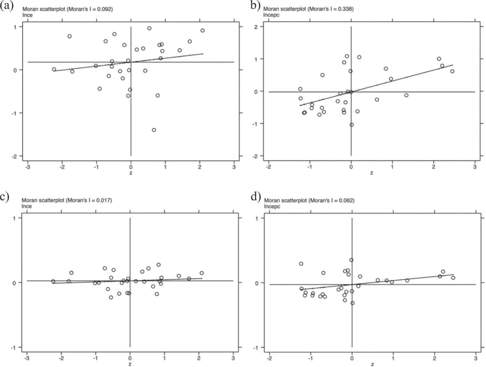
To measure the spatial correlation of provincial carbon emissions in China, we conduct both global and local spatial correlation tests. We calculate the global Moran’s I of provincial carbon emissions (measured by LnCE and LnCEPC) in the sample with the spatial weight matrices of WO and WI. The results show that the values of the global Moran’s I are significantly positive from 2008 to 2020, indicating a positive spatial correlation for carbon emissions among provinces.
Furthermore, we draw scatter plots of the local Moran’s I of provincial carbon emissions for 2019 with the spatial weight matrices WO and WI, respectively (see Fig. 2). We find that most of the scatter points are located in the first and third quadrants, while fewer scatter c) LnCEPC–WO, d) LnCEPC–WI. points are located in the second and fourth quadrants, indicating the characteristics of high–high and low– low agglomerations of provincial carbon emissions. Therefore, the use of the spatial econometric model is reasonable.
Model Selection
The common forms of spatial econometric models are the spatial lag model, the spatial error model, and the spatial Durbin model. The appropriate model specification can be ascertained on the basis of the Wald test, LR test, and LM test [29]. Table 4 presents the results of the statistical tests, where columns 1 and 2 take LnCE as the dependent variable and columns 3 and 4 take LnCEPC as the dependent variable. First, we test whether the spatial Durbin model can be simplified to the spatial lag model or spatial error model according to the results of the Wald and LR tests. The results show that the spatial lag terms and spatial error terms are not significant under WO and WI, indicating that we can expect a rejection of the spatial Durbin model in favor of the spatial lag model or spatial error model.
Furthermore, we can test whether the spatial lag model is more consistent with the sample data than the spatial error model based on the Lagrange multiplier (LM) test. Previous studies suggest that if the LM tests for spatial lag and spatial error have the same level of significance, then the model specification can be determined by the significance of robust LM tests [30]. The results presented in Table 4 show that the LM tests for spatial lag and spatial error are both significant at the 1% level, while the robust LM tests for spatial lag are more significant than those for spatial error. The tests on the relationship between green finance development and carbon emissions at the provincial level show that the spatial lag model is more acceptable on the data; thus, we use the spatial lag model in the following regressions.
Analysis of Spatial Lag Model
Table 5 presents the estimation results of the spatial lag models, where WO (columns 1, 3, 5, and 7) and WI (columns 2, 4, 6, and 8) are adopted as the spatial weight matrices, respectively.
We first use GF as the independent variable. The first four columns in the table show that the spatial-autoregressive parameters (rho values) are all significantly positive at the 1% level, indicating that an increase in carbon emissions in neighboring provinces will cause an increase in carbon emissions in the local province. These results further validate the positive spatial correlation of provincial carbon emissions. Therefore, carbon emissions need to be jointly prevented and controlled on a larger scale beyond the constraints of administrative boundaries. The coefficients of GF are significantly negative at the 1% level, preliminarily indicating that green finance development has a significant emission reduction effect.
Due to the spatial dependence on the dependent variables, we need to focus on the possible endogeneity problem in the regression models above. Wooldridge pointed out that if the error term of the model is only determined by the disturbance of the current period, then the endogenous variables lagged by one period in time can be used to replace the current value to deal with the endogeneity problems [31]. Considering that it is difficult to identify instrumental variables satisfying correlation and exogeneity for GF simultaneously, we introduce the variable L.GF into the model to mitigate the possible endogeneity problem and report the results in columns 5 to 8. For both matrices, the coefficients of the spatial lags of the dependent variables (rho values) are positive and significant, and the coefficients of L.GF are also negative and significant, indicating that the above results are robust.
Table 4.
Selection of spatial econometric models.
Table 5.
Green finance development and carbon emissions: spatial lag models.
[i] Note: Control variables include Urban, Openness, EI, LnGDPPC, and RD. The values in the table represent the regression coefficients in the spatial lag models. Rho from equation (2) represents the spatial-autoregressive parameter, which is the estimated coefficient of WlnCE (columns 1, 2, 5, and 6) or WlnCEPC (columns 3, 4, 7, and 8). *, ** and *** denote statistical significance at the 10%, 5% and 1% levels, respectively. Standard errors are given in parentheses.
Effect Decomposition
Due to the existence of a spatial lag term, the estimated coefficients of the variables in the spatial lag model cannot directly reflect their marginal effects (except for the spatial lag of the dependent variable) [29]. Therefore, we decompose the effects of green finance development on carbon emissions according to the partial differential methods proposed by LeSage and Pace [30].
Table 6 presents the direct, indirect, and total effects of green finance development on carbon emissions, in which we use GF (columns 1 to 4) and L.GF (columns 5 to 8) as the independent variables. The results show that green finance development on its own not only has a significant carbon emission reduction effect in the local province but also decreases carbon emissions in neighboring provinces. The direct effect is larger than the indirect effect when WO is used as the spatial weight matrix, while the direct effect is smaller when WI is used. One possible reason for this is that WO is the spatial adjacent weight matrix, which only reflects the spillover effects on the regions that are adjacent to the local region, while WI is the geographical distance weight matrix, which has a relatively loose limit on the geographical scope. Based on the theoretical analysis of the spatial correlation of carbon emissions, the competition, economic correlation, and demonstration effect are stronger between the spatially correlated regions in WO. Hence, the results with WO may be more consistent with the real situation in China, in which the direct effect of green finance development on carbon emissions is 1.6 times the indirect effect. The absolute values of the total effect of green finance development estimated by spatial econometric models are higher than those of the baseline regressions, indicating that the emission reduction effects are underestimated in the baseline regressions.
Heterogeneity Analysis
Due to differences in geographical environment, policy planning, and development goals, the emission reduction effect of green finance development might differ for different regions in China. Thus, we further test the heterogeneous effects in the eastern, central, and western regions of China and on both sides of the Hu Line. Direct cutting of the sample in spatial econometric models requires setting the spatial weight matrix separately, which may ignore some of the spatial effects. Therefore, we construct binary variables to indicate the regional location of the provinces and add their product terms with green finance development into the regressions.
The first four columns in Table 7 represent the direct effects of green finance development on carbon emissions. The results show that the carbon emission reduction effect of green finance development is more significant in the eastern and central regions compared to that in the western region. One possible explanation for this is that the level of financial development and marketization is relatively low in the western region. On the supply side, it is difficult for financial institutions to effectively use punitive and incentive measures to achieve an efficient allocation of financial resources. On the demand side, most companies have a low willingness to obtain green financial services due to their limited firm size.
The Hu Line (short for Hu Huanyong Line) is one of the greatest geographical discoveries in China. It divides the area of China into two parts-northwest and southeast-which are roughly equal in size but completely different in population density and economic activity. Columns 5 to 8 show that the carbon emission reduction effect of green finance development on the southeast side is significantly higher than that on the northwest side. In recent decades, more than 90% of China’s population and output have been concentrated on the southeast side of the Hu Line. China is planning to break through the Hu Line through a new type of urbanization. Some provinces on the northwest side propose to undertake industrial transfers from the southeast side. In this process, it is necessary to pay close attention to the structural effect of green finance development in the southeast, which may bring outdated production capacity to the northwest and lead to increased carbon emissions.
Table 6.
Direct, indirect, and total effects of green finance development on carbon emissions.
Table 7.
Direct effects for the heterogeneity analysis based on different regions.
[i] Note: The eastern, central, and western regions are determined according to the division criteria of the Seventh Five-Year Plan and Western Development strategy of China. Eastern (Central) is a binary variable taking the value of one if the province is located in the eastern (central) region, and otherwise, zero. Hu Line is a binary variable that takes the value of one if the province is on the southeast side of the Hu Line, and otherwise, zero. The values in the table represent the direct effects of the variables in the spatial lag models. *, ** and *** denote statistical significance at the 10%, 5% and 1% levels, respectively. Standard errors are given in parentheses.
Analyzing Mechanisms
We hypothesize that green finance development influences carbon emissions through two mechanisms: the technology effect of green technology innovation and the structural effect of industrial structure upgrading.
Table 8.
Direct effects for the mechanism analysis.
[i] Note: The values in columns 1 and 6 represent the regression coefficients in the fixed-effects models. The values in columns 2-5 and 7-10 represent the direct effects of the variables in the spatial lag models. *, ** and *** denote statistical significance at the 10%, 5% and 1% levels, respectively. Standard errors are given in parentheses.
Since the mechanism analysis mainly focuses on the influences of the local independent variables and mediating variables on their dependent variables, we report only the direct effects of the key variables in the spatial lag models. Table 8 displays the results from fixed-effects regressions (columns 1 and 6) and spatial lag models (columns 2-5 and 7-10). We test the technology effect and structural effect of green finance development in Panels A and B, respectively. Column 1 in Panel A shows that green finance development will significantly promote green technology innovation. With the spatial weight matrices WO and WI, the coefficients of GTI in columns 2 to 5 are all negative and significant, indicating that China’s green invention patents can be effectively transformed into green productivity and that green technology innovation has become an important driving force for carbon emission reduction. In summary, green finance development reduces carbon emissions by promoting green technology innovation, and thus, the mechanism of the technical effect of green finance development is verified.
Since the twenty-first century, China’s economy has gradually transformed from industrialization to service industries. In the context of economic restructuring and supply-side reform, the optimization of the industrial structure is still a key direction in an era of structural adjustment. Therefore, it is of great practical significance to clarify the impact of industrial structure upgrading on carbon emissions in China. Column 6 in Panel B shows that green finance development contributes to the transformation of the industrial structure from the secondary industry to the tertiary industry. Columns 7 to 10 show a highly negative relationship between industrial structure upgrading and carbon emissions, which indicates that the further green upgrade of the industrial structure is a solution to promote low-carbon transformation and development in China. The above analysis demonstrates that green finance development reduces carbon emissions by promoting industrial structure upgrading and reveals the underlying mechanism of the structural effect.
Evidence from China’s Carbon Emissions Trading Policy
Carbon finance, as a key area of green finance, plays an important role in promoting energy structure transition and low-carbon development [32]. In the process of evaluating green finance development, indicators for new financial markets, such as carbon finance, should be considered along with the traditional financial market indicators, such as credit, securities, and insurance. As for the governance of carbon emissions, the Chinese government has been making continuous efforts to address global climate change through market-incentivized environmental regulations, such as carbon emission trading. Carbon emission trading refers to building an emission trading market in which enterprises, with consideration of their production, are granted a certain amount of carbon quotas that they can buy and sell freely. With the release of the Notice on Pilot Work of Carbon Emissions Trading issued by the National Development and Reform Commission of China, the carbon emission trading policy has been officially launched in seven provinces and cities (including Shanghai, Beijing, Guangdong, Shenzhen, Tianjin, Chongqing, and Hubei) in China since 2012. Carbon emission trading has developed rapidly in recent years and has become an important measure for China to achieve its dual-carbon goals. Theoretically, the Coase Theorem suggests that the clarity of property rights can increase the efficiency of resource allocation. Trading carbon emission rights as commodities among enterprises has an effective emission reduction effect because buying quotas in the trading market will internalize the externality cost of carbon emissions generated by production activities, and enterprises are motivated to reduce energy consumption by using clean energy or equipment.
Table 9.
Test of parallel trend assumption.
Due to the limited time, the carbon emission trading data cannot be matched with the previous sample interval, so the dimension of carbon finance is not included in the aforementioned indicator system of green finance development. Therefore, we use China’s carbon emission trading policy as a quasi-natural experiment to investigate the impact of carbon finance on carbon emissions. We take 2012 as the point of policy implementation. By incorporating the spatial lag of the dependent variable into the difference-in-differences (DID) model, we estimate the following SLM-based SDID model:
where Treati is a binary variable taking the value of one if province i is included in the pilot, and otherwise, zero. Postt is a binary variable that equals 1 if year t is after 2012, and otherwise, zero. The coefficient of the interaction term Treati×Postt measures the treatment effect of the carbon emission trading policy.
Table 10.
Carbon emission reduction effect of China’s carbon emission trading policy.
[i] Note: Control variables include Urban, Openness, EI, LnGDPPC, and RD. The values in the table represent the direct or indirect effects of the variables in SDID models. *, ** and *** denote statistical significance at the 10%, 5% and 1% levels, respectively. Standard errors are given in parentheses.
Table 11.
Robustness checks.
[i] Note: The values in the table represent the regression coefficients in the spatial lag models. Rho from equation (2) represents the spatial-autoregressive parameter, which is the estimated coefficient of WlnCE (columns 1, 2, 5, 9 and 10), WlnCEPC (columns 3, 4, 6, 11, and 12), or WlnCEI (columns 7 and 8). *, ** and *** denote statistical significance at the 10%, 5% and 1% levels, respectively. Standard errors are given in parentheses.
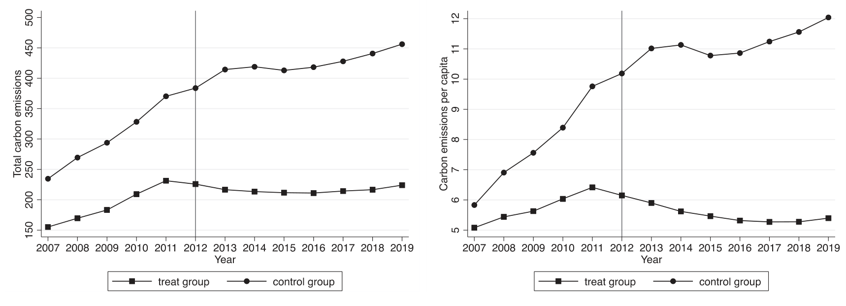
The premise of using the DID model is that the data satisfy the parallel trend assumption; otherwise, we cannot obtain consistent estimators from the DID model. Fig. 3 plots the group averages of total carbon emissions and carbon emissions per capita for the treatment group (Treati = 1) and control group (Treati = 0) from 2008 to 2020. Taking the year of policy implementation (2012) as the time node, the results show that the carbon emission trends of the treatment and control groups were roughly the same before 2012. However, there was a significant difference in the trend between the two groups after 2012. Therefore, it can be tentatively concluded that the samples we use satisfy the parallel trend assumption.
We further test the parallel trend assumption by constructing regression models based on the method proposed by Autor et al. [33]. We construct time binary variables Dk for each of the four years before and after 2012 and put their product terms with Treat into the regressions. As mentioned above, the coefficients of the spatial lag model do not reflect their marginal effects. Thus, we present the direct effects of the interaction terms (Treat×Dk) in Table 9, which refer to the overall effects of the variables on local carbon emissions. The results show that the direct effects of Treat×Dk (k = -4, -3, -2, -1) are not significant, thus confirming the parallel trend assumption.
We test the carbon emission reduction effect of the carbon emission trading policy by using SDID models and present the empirical results in Table 10. The direct and indirect effects of Treat×Post are all negative and significant with either one of the spatial weight matrices WO or WI, indicating that China’s carbon emission trading policy could not only reduce carbon emissions in the pilot provinces but also restrain carbon emissions in the neighboring provinces. Moreover, the direct and indirect effects of GF are all significantly negative, which is consistent with the previous results.
Robustness Checks
For the robustness checks, we turn to an alternative method to measure green finance development. We construct an independent variable GF_GPCA based on the global principal component analysis (GPCA) and include it in the model. Principal component analysis (PCA) is a popular technique that reduces the dimensions of originally correlated random variables into new comprehensive variables that are independent of each other through orthogonal transformation. GPCA extracts PCA by considering the dynamic changes in variables, which is more applicable when analyzing the panel data. The first four columns in Panel A of Table 11 display the regression results obtained from spatial lag models with the independent variable GF_GPCA. The coefficients of green finance development are significantly negative. We also find that a significant positive spatial correlation exists in carbon emissions among provinces, indicating the robustness of the previous results.
Special attention should be paid to the setting of the spatial weight matrix when estimating a spatial econometric model. We construct another geographical distance weight matrix based on highway distances (WU) to replace the spatial weight matrices used in the previous models. Based on the highway information of China, we calculate the highway distance between the capital cities of any two provinces and use the inverse of highway distance as the spatial weight. The results in columns 5 and 6 in Panel A show that green finance development is negatively related to carbon emissions after replacing the spatial weight matrix. We also find that the spatial-autoregressive parameters (rho values) are significantly positive at the 1% level, which is consistent with the previous results.
Considering the level of economic development, we replace the dependent variable with the natural logarithm of carbon emission intensity (LnCEI), which indicates the carbon emissions per unit of GDP. The regression results obtained from spatial lag models after replacing the dependent variable remain the same (see columns 7 and 8 in Panel B of Table 11).
Considering the comparability of the sample, we exclude the observations of municipalities (including Beijing, Shanghai, Chongqing, and Tianjin) from the sample and only retain those of provinces and autonomous regions for robustness checks. The regression results are shown in columns 9 to 12 in Panel B, which are compatible with the previous analysis.
Conclusions
In this paper, we investigate the relationship between green finance development and carbon emissions using the provincial panel data in China and draw the following conclusions: (1) Because of the competition, economic correlation, and demonstration effect, there is a positive spatial correlation of carbon emissions among provinces in China. The increase in carbon emissions in neighboring provinces positively affects carbon emissions in the local province. (2) Green finance development on its own not only has a significant carbon emission reduction effect in the local province but also decreases carbon emissions in neighboring provinces. In addition, it reduces carbon emissions through two mechanisms: the technology effect of green technology innovation and the structural effect of industrial structure upgrading. (3) The carbon emission reduction effect of green finance development exhibits regional heterogeneity. The effect is more pronounced in the eastern and central regions than in the western region. Moreover, the effect on the southeast side of the Hu Line is significantly higher than that on its counterparts.
(4) Further analysis shows that China’s carbon emission trading policy also has a significant negative effect on carbon emissions in the pilot provinces and their neighboring provinces.
In general, the results of this paper deepen the research related to carbon emission reduction driven by green finance development and provide some important policy implications for effectively promoting low-carbon transformation and development.
First, as a cross-regional public good, the environment has obvious externalities. Due to the positive spatial correlation of carbon emissions, the policy instruments that aim to achieve the low-carbon transformation of economic development will inevitably have indirect effects on other provinces through geographical and economic connections. Thus, a long-term mechanism of carbon emission regulation should be built across administrative boundaries for joint prevention and control. In addition, corresponding policies should be introduced to encourage enterprises to form green alliances across administrative regions to promote the optimal allocation of green production factors among regions.
Second, since the carbon emission reduction effect of green finance development differs for different regions in China, a “one-size-fits-all” approach should be avoided when formulating energy conservation and emission reduction policies. In the process of new urbanization, it is necessary to pay close attention to the structural effects of green finance development in the eastern and central regions, as well as the southeast side of the Hu Line. Such an effect may lead to the accelerated transfer of two high and one low industries (high pollution, high energy consumption, and low capacity) to the other regions of China.
Third, since the promotion of green technology innovation will effectively reduce carbon emissions, public policy might consider providing necessary incentives for green technology innovation through effective institutional arrangements of green finance. Innovation ability in key areas can be enhanced by formulating a dynamically adjusted guiding catalog of green technologies, establishing special funds for green innovation, and offering loans at subsidized interest rates to enterprises that actively carry out green R&D activities.
Fourth, our results demonstrate that the optimization and adjustment of industrial structures should be guided by efficient green financial policies to reduce carbon emissions. The industrialization and urbanization processes in China are characterized by high energy consumption and high emissions. The coal-based energy consumption structure has exerted a lock-in effect on the negative environmental externalities of economic development. On one hand, it might be beneficial to reduce the carbon emissions of existing industries with high energy consumption and high emissions by strengthening energy and environmental constraints. On the other hand, by increasing the environmental access threshold, domestic and international capital will be guided to flow to low-carbon sectors to curb carbon emissions.