

Introduction
Territorial space [1-4] is a complex and extensive system, shaped by the interactions, interplays, infiltrations, and couplings of various elements such as nature, economy, society, and human activities. It serves as the venue for a country's political, economic, and cultural activities and acts as the foundation for diverse construction projects. Faced with challenges including tightening resource constraints, worsening environmental pollution, and ecosystem degradation, the 18th National Congress of the Communist Party of China proposed optimizing the territorial space by constructing a "triple-bottom-line space." The 19th National Congress further emphasized the need to demarcate three control lines: ecological protection redlines, permanent basic farmland, and urban development boundaries, aiming to adjust and optimize the structure of the territorial space.
With the 2019 release of the "Opinions on Establishing a National Spatial Planning System and Supervising its Implementation" by the General Office of the Communist Party of China Central Committee and the General Office of the State Council, territorial spatial planning has been formally established as a leadership role and top-level directive across all types of spatial planning. It is expected to resolve the issue of overlapping and contradicting objectives and contents of various spatial plans, leading to the integration and unification of multiple regulations. The central leadership consistently emphasizes adherence to bottom-line thinking, using territorial spatial planning as a basis for adjusting economic structures, planning industrial development, and promoting urbanization. Urban areas, agriculture, and ecological spaces, along with their respective protection red lines, are considered insurmountable boundaries that play a strategically important role in the economic and social development of the country through national land spatial planning.
To support the national strategy, scholars have conducted relevant research. Utilizing global surface coverage data and building on existing classification methods for national land use, researchers propose dividing land space into three categories: agricultural, urban, and ecological spaces. Building on the theoretical foundations and conceptual frameworks of these three life spaces, Lin Gang et al. [5] highlighted the integrated and coordinated use of production, living, and ecological spaces. They introduced a conceptual framework consisting of four elements: spatial structure, functional zoning, ecological protection, and social participation, drawing from both domestic and international research findings. Further, Ji Zhengxin et al. [6] applied a multifunctional value assessment methodology to identify and regulate the spatial patterns of these living spaces, with Zhangjiakou City serving as a case study. In exploring the evolution of spatial and temporal patterns of national land use, Shawky Mansour et al. [7] employed cellular automata and geospatial technology to evaluate and predict urban growth and changes in land cover. Additionally, Xu Zhirong et al. [8] used GIS-based spatial distribution and statistical models to characterize the evolution of spatial distribution and the influence of various factors on the spatio-temporal patterns of settlements. M. Munthali et al. [9] engaged in focus group discussions, key informant interviews, and semi-structured interviews with 586 households to identify drivers of land use and land cover change (LULC). ZHU W et al. [10] applied entropy-weighted TOPSIS and Tobit modeling to examine the spatial and temporal evolution patterns and spatial correlations of 13 cities in Jiangsu Province, analyzing the drivers of benefits from these patterns. Generally, existing studies emphasize the spatial and temporal evolution of land under natural and human influences, but pay less attention to the influences of economic and policy factors.
Regarding the classification system [11-13], understanding the formation mechanisms of national land space and its interrelationships across production, life, and ecology is fundamental for classifying and optimizing national land space structures, a view widely accepted by academics. However, the categorization of "ecological-agricultural-urban space" within national land spatial planning is rarely addressed. Research primarily focuses on urban agglomerations and administrative divisions across local or global scales [14-16], with analyses ranging from micro to macro perspectives of national land space evolution and function. Yet, in-depth analyses at the meso-level, which combine watershed and administrative divisions, particularly in ecologically vulnerable areas where land, rivers, and oceans converge, are infrequently conducted. In terms of methods for analyzing spatial and temporal evolution [17-20], the land-use transfer matrix [21, 22] and landscape pattern index [23-25] are crucial for depicting the evolution of national land space. These methods can quantitatively demonstrate the relationship between spatial evolution and its structure. However, the evolution of land involves not only quantitative changes but also the dynamics of speed and spatial attributes, particularly the spatial expression of agglomeration or disaggregation. Such quantitative relationships between neighboring administrative units are rarely reported.
This study is dedicated to the sustainable development of the region, taking the Hanjiang River Basin as the focal area. Utilizing land cover, social, and humanities data from 2000 to 2020, it builds upon and refines previously researched spatial categorization systems. The study delineates the spatial evolution of the land in multiple dimensions, including processes, patterns, and driving factors, to comprehensively uncover the general principles of land evolution. This, in turn, aims to provide decision-making references for the region's spatial planning and high-quality development.
Overview of the Study Area and Data Sources
Overview of the Hanjiang River Basin
The Hanjiang River Basin is situated in eastern Guangdong, southwestern Fujian, and southern Jiangxi, encompassing 8 prefecture-level cities and 24 counties (cities and districts) (Fig. 1). The upper and middle reaches of the region are sparsely populated, whereas the lower reaches and delta are densely populated, with Shantou having the highest density. In 2020, the watershed had a GDP of 2090.2 billion yuan, indicating a relatively developed economy. The main stream spans 470 km and covers a basin area of 130,803 km², with 36,812 km² (28.14%) in Guangdong Province, 54,626 km² (41.76%) in Fujian Province, and 39,365 km² (30.10%) in Jiangxi Province. The Meijiang River is the mainstream of the Han River, originating at the junction of Zijin County and Luhe County in Guangdong Province. It has a length of 307 km and an average gradient of 0.40%, covering a catchment area of 13,929 km². The largest tributary, the Ting River, originates from Laijiashan in Ninghua County, Sanming City, on the southeast side of the southern section of Wuyi Mountain. It extends 322 km, with an average gradient of 1.5%, and spans a catchment area of 11,802 km².
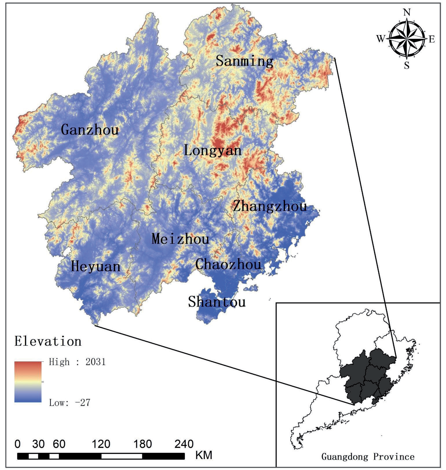
The basin frequently experiences floods and droughts, serious water pollution in some river sections, and common soil erosion in the mountainous and hilly areas of the upper and middle basin, necessitating significant governance and protection efforts. In October 2020, General Secretary Xi Jinping, during his visit to Chaozhou, emphasized the importance of comprehensive management of the Han River basin to ensure its long-term clarity. In 2021, the Pearl River Water Resources Commission of the Ministry of Water Resources drafted a "comprehensive plan for the Hanjiang River Basin", establishing four major systems for flood prevention and disaster mitigation, water resources conservation and utilization, water ecological environmental protection, and comprehensive basin management. Efforts in comprehensive management are now showing results, with several targets for 2025 being achieved ahead of schedule.
Data Sources and Data Processing
The dataset comprised data from the years 2000, 2005, 2010, 2015, and 2020, analyzed in five-year intervals. This selection allows for the systematic observation and analysis of long-term trends and changes. The overview data for the Han River Basin are sourced from several plans and programs, including the Han River Basin Comprehensive Plan, the Guangdong Province Han River Basin Comprehensive Water Conservancy Management Work Programme, and the Gan, Fujian, and Guangdong Former Central Soviet Areas Revitalization and Development Plan. Specific data for each city are derived from their respective statistical yearbooks: Meizhou (2000), Shantou (2005), Chaozhou (2010), Heyuan (2015), and Zhangzhou (2020), along with the Longyan, Ganzhou, and Sanming Statistical Yearbooks. Initially, remote sensing data were extracted using the boundary of the study area to form the foundational database for the land space in ArcGIS 10.3. The land space was then classified into three levels based on the correspondence between the LUCC classification system and the land space, as shown in Table 1.
Land cover data were processed using the boundaries of the study area. Based on the CLCD classification system and the correspondence of the national land space, the land was refined into three levels of classification (illustrated in Table 1). Social and humanistic attributes were integrated into each raster unit using GIS software, creating a spatio-temporal database for the national land space classification that serves as the foundation for the analysis and research presented in this study.
Table 1.
Spatial classification system of land in the Han River Basin.
Research Methodology
String Diagram Visualization Models
A string diagram visualization model is a data visualization technique that displays interrelationships between data arranged in a matrix. This method is primarily used to illustrate the relationships among multiple objects [26]. The string diagram consists of nodes and strings: nodes are arranged radially along the circumference of a circle, and chords, which are arcs weighted by width, connect any two points on the circle. Each chord represents the correlation between the two points. Nodes and chords are differentiated by color, allowing for a visual comparison of data and making it highly suitable for representing complex relationships. The number of nodes in the chord diagram reflects the current number of targets; the contact area between the arc and the node (the thickness of the chord) indicates the degree of relationship or proportionality between two sets of data, and the color of the arc can match either the target node or the source node.
Geological Information Mapping
Geological information mapping involves the use of extensive digital resources, including remote sensing, map databases, GIS, and digital earth technologies [27]. This process uses graphical concepts and abstract reasoning, along with computer three-dimensional and dynamic visualization technologies, to illustrate the characteristics and patterns of the earth system and its elements across space and time. The primary purpose of geological information mapping is to visualize changes in the quantity and type of land space, facilitating the depiction of transformations from one land space type to another.
In this study, land cover data from two different years are overlaid using GIS software according to Equation 1. The resulting data are then reclassified to depict both the upward and downward transitions of land space types. The formula is as follows:
In Equation (1), X represents the national spatial map obtained through raster calculations, Q represents the national spatial map from two distinct years with the earlier year noted first, and H represents the national spatial map with the later year. For example, X=13 signifies the transformation of green ecological space into rural production space. After extraction and reclassification, this indicates a downward trend in the green ecological space and an upward trend in the rural production space.
Center of Gravity Offset Modeling
The center of gravity shift model calculates the coordinates of the mean center for each type of land space annually and then uses these coordinates to track the trajectories of shifts in different land spaces [28]. This model enables the calculation of the spatial distribution of each land space type, facilitating analysis of land space transfers across various regions.
The model visualizes the trajectory of land space changes, showcasing the migration of land space centers of gravity over different periods. The calculation formulas are as follows:
In Equations (2) and (3), P and Q represent the coordinates of the centers of gravity for different territorial spaces; Tb and c denote the total area (km2) and the number of areas of the bth region; and Lb and Fb represent the coordinates of the center of gravity of the bth region.
Spatial Autocorrelation Analysis
Spatial autocorrelation analysis examines whether there is a connection between changes in the same type of land space across different regions or between changes in one type of land space and changes in another. This analysis is divided into univariate and bivariate spatial autocorrelation [29-31]. Univariate spatial autocorrelation is formulated into the following functions:
In Equations (4) and (5): C represents the univariate spatial autocorrelation index; Oi and Ot are the land changes in the vth and tth plots, respectively; b is the number of regions; Fit is the spatial weight matrix; O is the spatial mean of the amount of change; S(I) is the standardized statistic threshold; E(I) is the expected value of the autocorrelation of the observed variables; and var(I) is the variance. The values of C range between [-1, 1], with C >0 indicating a positive relationship in the amount of land change.
The formula for bivariate spatial autocorrelation is as follows:
In Equation (6): LiAB denotes the bivariate local spatial autocorrelation coefficient for geographic patch i; XiA indicates the amount of change in land category A for geographic patch i; XiB is the amount of change in land category B for geographic patch i;
Geoprobes
Geoprobes are a suite of statistical methods designed to detect spatial variation and identify the driving forces behind it. The premise is that when a variable significantly influences a dependent variable, their spatial distributions should be similar [32]. Geodetectors treat the factor under study as the independent variable and the factor to be detected as the dependent variable. As the units of each data set are different, the rate of change of each data set is used as the indicator. Through discretization, these are classified into five categories according to natural classification. Spatial autocorrelation helps identify the factors that most significantly affect the process of spatial change in the country, allowing for targeted policy adjustments to mitigate unfavorable impacts and favorable ones.
Table 2.
Indicators of the drivers of the spatial evolution of the homeland.
The formula is as follows:
In Equation (7): Q is the driving detection indicator in the process of land evolution; L is the total number of samples in the study area; nt is the total sample size; t is the number of variables; δ2is the total variance within the study area; δt2 is the discrete variance. The value interval of Q is [0, 1], where Q=0 indicates that the elemental factor is randomly distributed; the larger the value of Q, the greater the influence of the testing factor in driving the spatial evolution of the land. Based on these theories and typical cases, and in conjunction with the actual situation of the Hanjiang area, evaluation indexes are established from five aspects: natural environment foundation, transportation location conditions, social living conditions, economic development level, and policy and institutional environment (Table 2).
Results and Analysis
Characterization of the Overall Spatial Evolution of the National Territory
The land cover data of the study area were categorized according to land space classification (Table 3). From 2000 to 2020, the findings include:
The ecological space consistently covered more than 106,307 km2, accounting for over 80% of the total area, marking it as the predominant land type.
Agricultural space remained stable at approximately 22,067 km2, representing more than 17% of the land.
Urban space increased significantly, rising from 788 km2 in 2000 to 2,585 km2 in 2020, yet it still accounted for the smallest proportion, about 1%.
Over the 20 years, the spatial changes for these three types of land were as follows:
Ecological space decreased by 982 km2 (approximately -1%),
Agricultural space decreased by 761 km2 (about -3%),
Urban space expanded by 1,797 km2 (an increase of 228%).
The most substantial change occurred in urban areas, particularly between 2000 and 2005, indicating rapid urban expansion during this period. Policy adjustments, particularly increased ecological awareness and the implementation of arable land protection strategies, have slowed the encroachment of urban areas into agricultural and ecological spaces.
From the data on the changes in different types of land use (Table 3), both ecological and agricultural spaces have shown a consistent decreasing trend over the years, whereas urban space has been increasing annually. However, the decrease in ecological and agricultural spaces is less noticeable since they constitute a large portion of the total area. In contrast, the growth of urban space is quite pronounced due to its initially small percentage. For instance, in 2000, urban space was only 788 km², but by 2005, it had increased by 683 km², marking an 87% growth rate, while ecological space decreased by 590 km², which is less than 1%. Further analysis indicates a rapid increase in urban living space and industrial and mining production space. Meanwhile, rural agricultural production has been declining annually, and rural living space has generally been increasing. Ecological space trends are similar to those of agricultural space, with the green cover ecological space diminishing each year, while water ecological space first increased and then decreased.
Table 3.
Statistical table of spatial changes in the Hanjiang River Basin from 2000 to 2020.
Overall, the national land use in the study area exhibits an irreversible trend toward increasing urban space, thereby reducing ecological and agricultural spaces. This trend aligns with the rapid economic development and urbanization that demand substantial urban land [33].
Analysis of the Process of Spatial Evolution of the National Territory
Characterization of Size
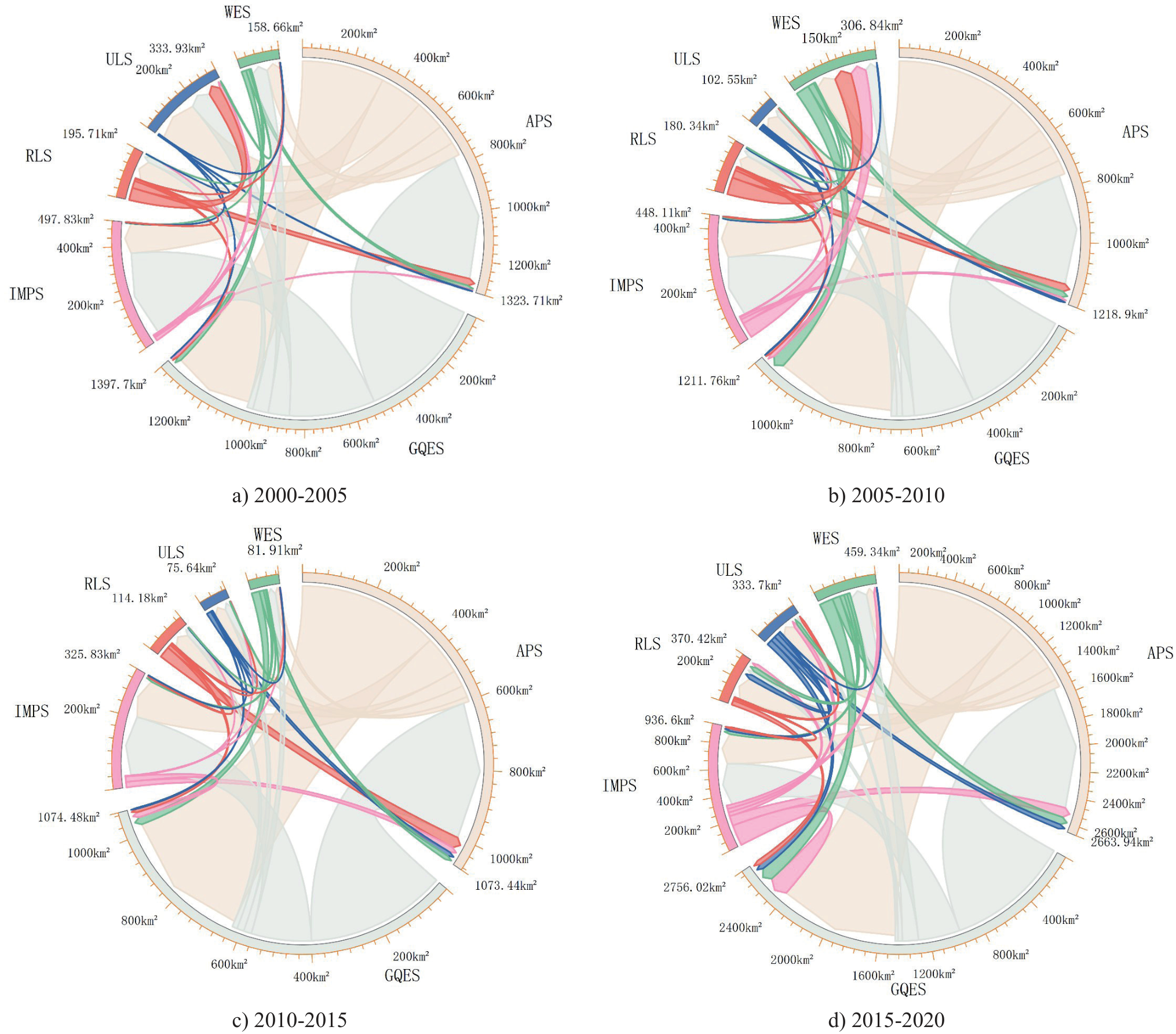
Using the chordal graph visualization model, the scale characteristics of land space changes in the study area at different stages were analyzed. From 2000 to 2005 and from 2005 to 2010, the changes were predominantly marked by the encroachment of industrial and mining production space on green ecological areas and the transformation of rural production space into other uses. From 2010 to 2015, this encroachment and transformation slowed down, with a marked increase in the conversion of rural production space and green ecological areas. From 2015 to 2020, the space dedicated to agricultural production significantly increased, while the transformation of rural production space and green ecological areas markedly decreased. Over the past 20 years, the changes in land space in the study area have primarily involved the conversion of agricultural and ecological spaces into each other and into urban space (Fig. 2).
Spatial Mapping Characterization
(Ⅰ) Basic change mapping
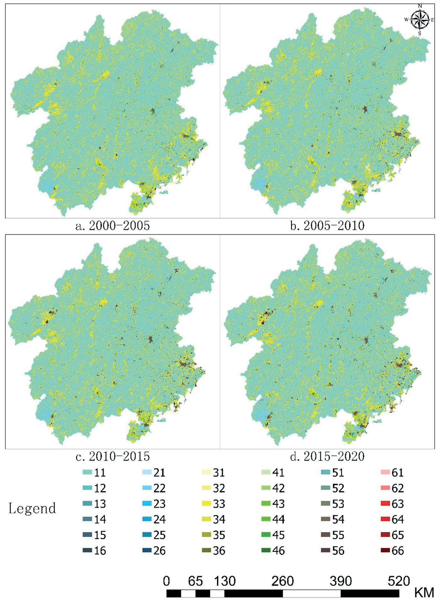
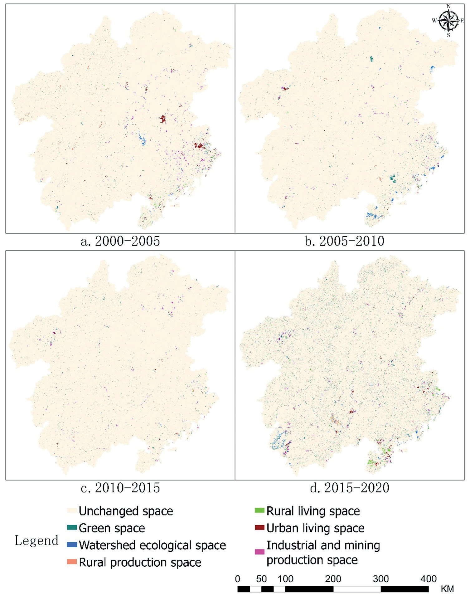
The spatial mapping analysis revealed that a total of 60 mapping units underwent changes from 2000 to 2005 (Fig. 3a), with the transition from "green cover ecological space to rural production space" (code 13) being the most prevalent. The shift from "green cover ecological space to industrial production space" (code 16) was notably concentrated in Zhangzhou City and Longyan City. The most prominent changes from 2005 to 2010 (Fig. 3b) involved the same categories (code 13 and code 31), which represent internal transitions between green cover ecological space and rural production space, showing a broader distribution. The mapping unit changes from 2010 to 2015 were similar to those from the previous period (Fig. 3c). The period from 2015 to 2020 (Fig. 3d) also displayed internal transitions between green cover ecological space and rural production space, but these transitions increased significantly in frequency and were more spatially dispersed. Overall, throughout the 20-year study period, the three types of land space in the study area experienced significant changes, with 60 units altering and the most frequent transformations occurring between green cover ecological space and rural production space.
(Ⅱ) Mapping of upward and downward trend changes
Fig. 2.
Visualization of the chord diagram of spatial changes in the land. Note: IMPS, ULS, RLS, APS, WES, and GQES represent industrial and mining production space, urban living space, rural living space, agricultural production space, water ecological space, and green ecological space, respectively.
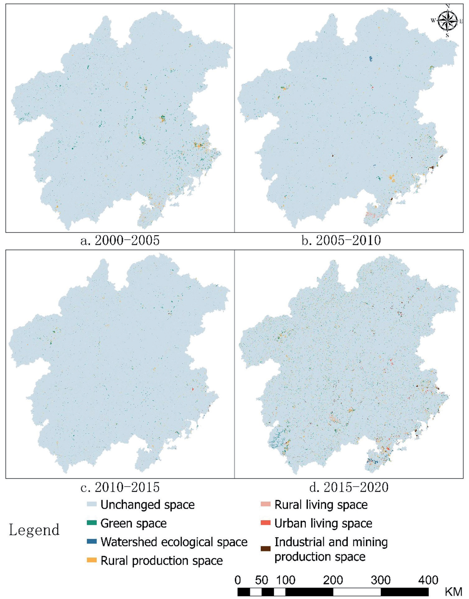
From the analysis of the fall potential mapping (Fig. 4), the change in fall potential from 2000 to 2020 was relatively stable, but the distribution of these changes was complex and widespread. During 2000-2005, the area of fall potential change accounted for less than 1% of the total area, predominantly involving green cover ecological space and rural production space, concentrated in Longyan City. The fall potential change from 2005-2010 was similar overall to the previous period, with the area of change being less than 1%, primarily due to the reduction in industrial and mining production space in Chaozhou and Shantou. The trend from 2010-2015 followed a similar pattern, with fall potential changes mainly transitioning from rural production to other types of land use, concentrated in Ganzhou City. From 2015-2020, there was a significant increase in fall potential changes, mainly attributed to the heightened dynamics in urban living spaces in Heyuan and Shantou.
According to the rising trend mapping (Fig. 5), the entire study period predominantly featured internal conversions between green ecological space and rural production space. The most pronounced rising trend was in urban living spaces. From 2000-2005, the area of change was stable at 1%, with the most notable rise observed in urban living space, concentrated in Zhangzhou City and Longyan City, largely transitioning from green ecological space. From 2005 to 2010, there were no significant changes in the spatial status of the land, with urban living space continuing to show a prominent increase, now shifting from the central part of Zhangzhou City to the coastal areas. From 2010- 2015, the general trend remained consistent, with urban living space still prominent, although the rate of increase slowed and the spatial distribution became more dispersed. From 2015-2020, the rising trend in the change area increased significantly, accounting for 3%, with the most distinct increases in rural production space and green cover ecological space. The rise in urban living space also saw a considerable increase. Generally, before 2010, the most noticeable increase was in urban living space, aligning with China's rapid economic development and accelerated urbanization during that period. After 2010, the most significant and extensive increases were in rural production space and green ecological space, closely related to China's policy adjustments focused on ecological environment protection and arable land conservation [34].
Fig. 3.
Mapping of spatial changes in the national territory, 2000-2020. Note: The map unit represents the transformation of territorial space type, with the code consisting of two secondary classification codes of the transformation. For example, "ecological space of water area → industrial and mining production space" (Code 26).
Analysis of Spatial and Temporal Patterns of Territorial Spatial Evolution
Trajectory Analysis of Territorial Spatial Evolution
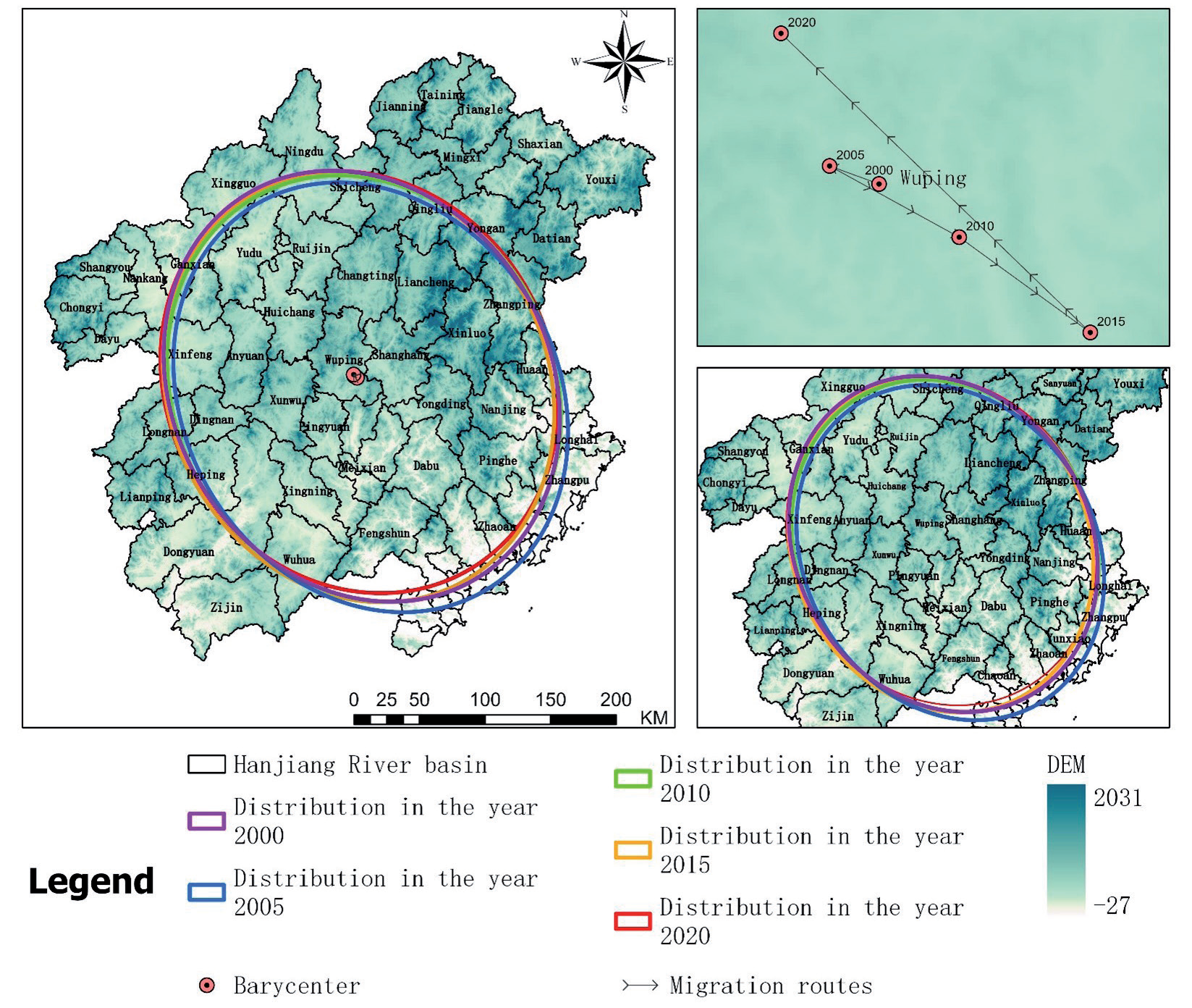
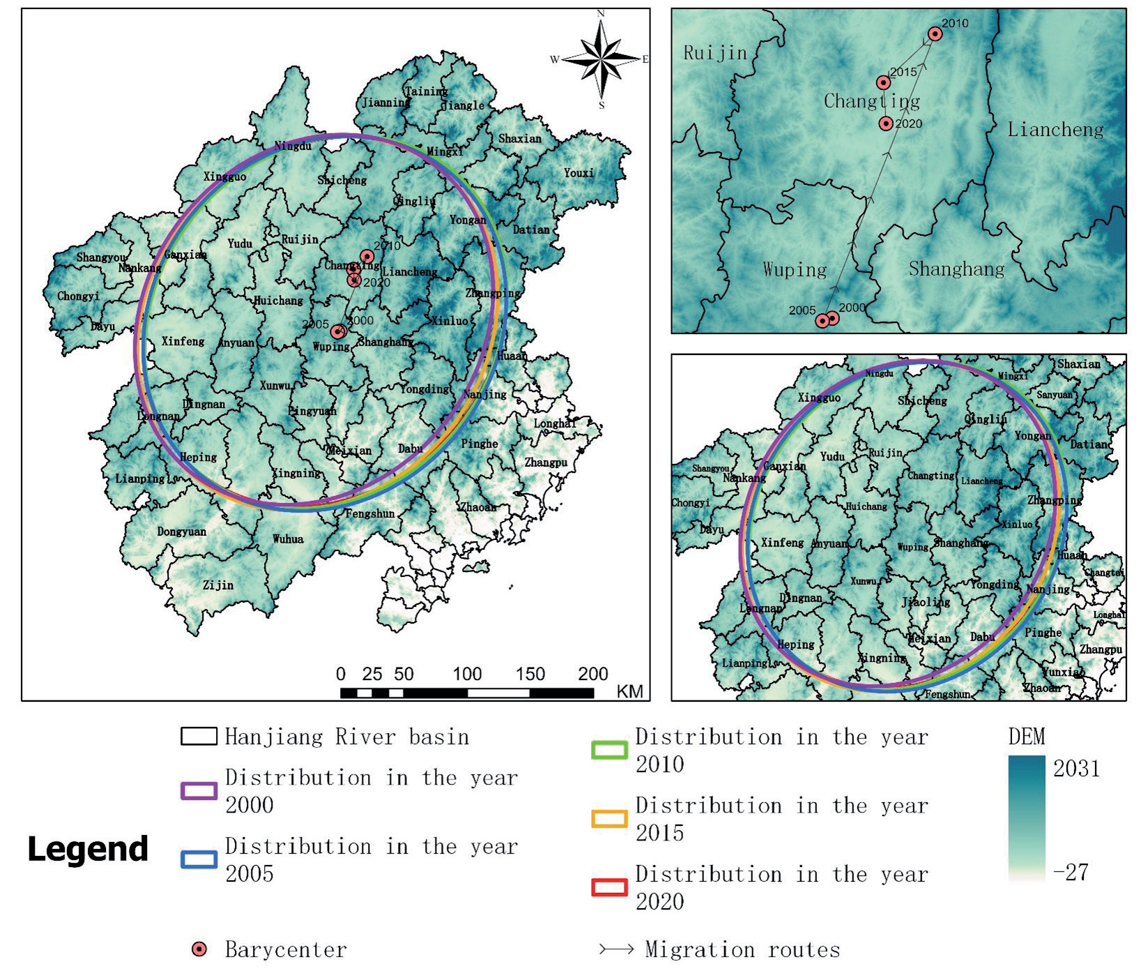
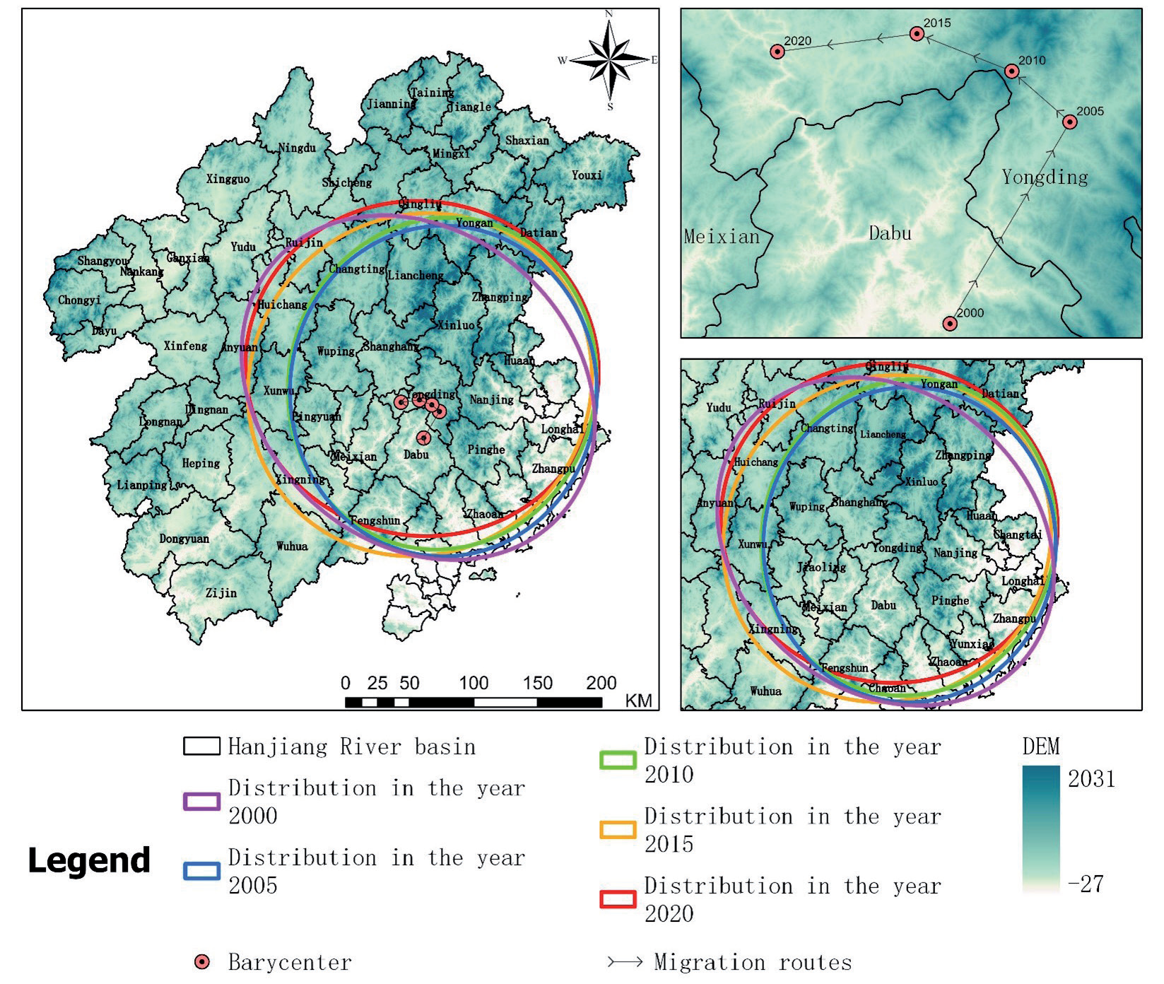
Using the center of gravity shift model, we calculated and visualized the center of gravity for the three types of land space in the study area across different years (Figs. 6-8). The center of gravity for ecological space is located in Wuping County, Longyan City. It shifted from the northwest to the southeast during 2000-2015 and then reversed direction from 2015-2020, ultimately surpassing its initial position in 2000. The center of gravity for agricultural space, situated in Wuping County and Changting County in Longyan City, displays an overall northeast-southwest from southwest to northeast from 2000 to 2010 and then meandered from northeast to southwest from 2010 to 2020, nearing its original position in 2000. The center of gravity for urban space, located in Wuping County in Longyan City and Tai Po County in Meizhou, shifted from southwest to northeast from 2000-2005 and then from southeast to northwest from 2005-2020.
The main reason for the varying centers of gravity among the three spatial types in different periods is the disparate levels of economic development and urbanization among the cities in the study area. Each city and county is at a different stage of development during the same period, which causes deviations in the centers of gravity [35].
Territorial Spatial Autocorrelation Analysis
(Ⅰ) Univariate
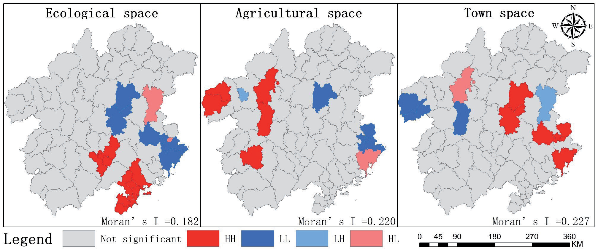
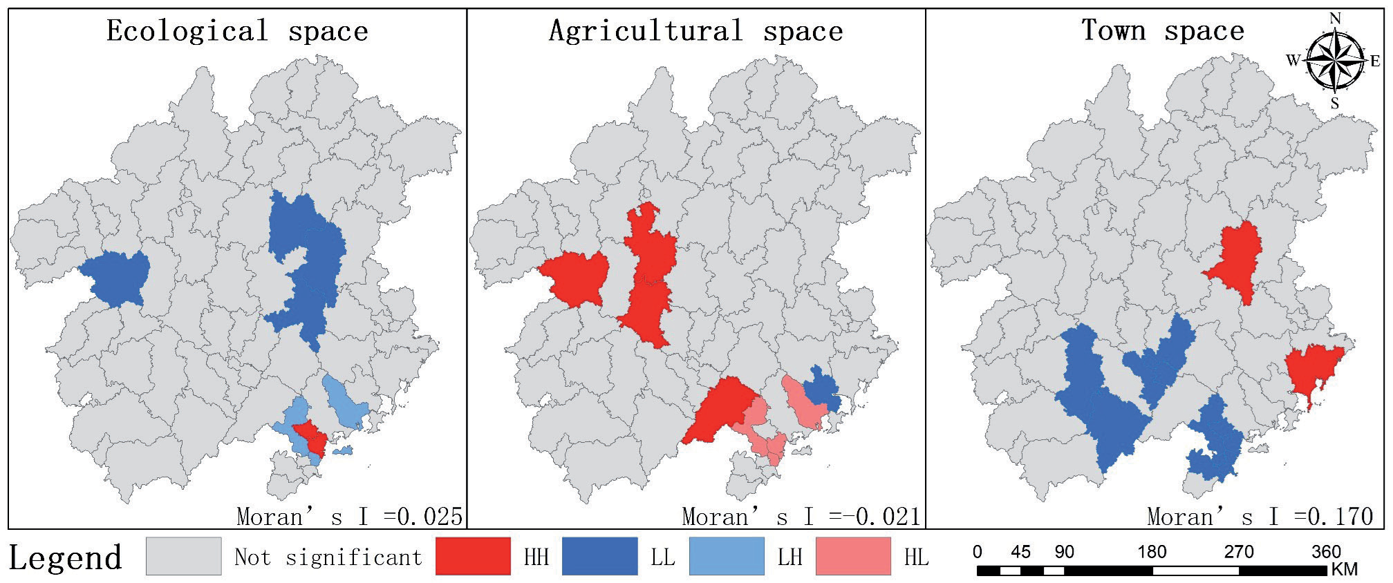
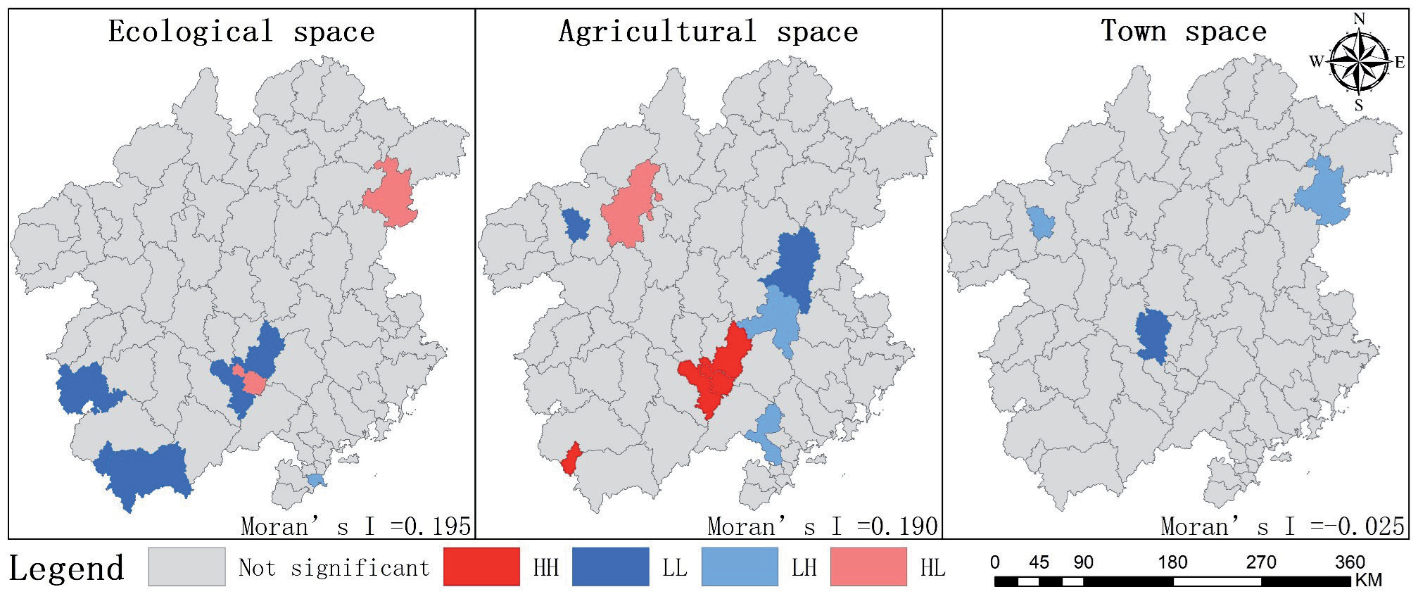
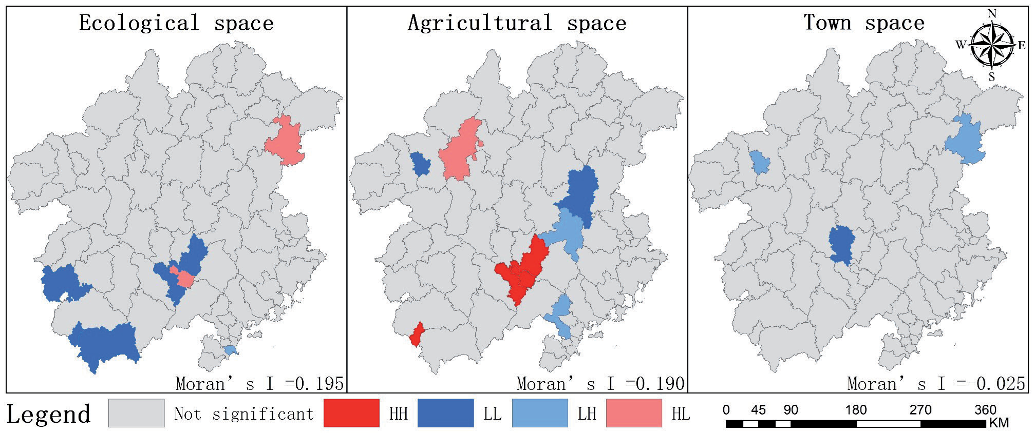
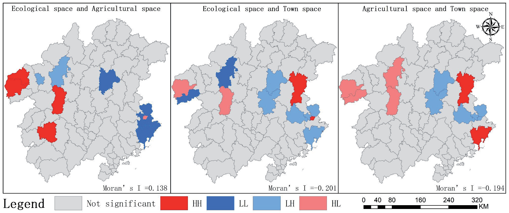
In the univariate spatial autocorrelation analysis (Figs. 9-12), apart from the Moran's I index for urban space in 2010-2015 and 2015-2020, and for agricultural space in 2005-2010 which were less than 0 indicating a negative correlation, the rest of the Moran's I indices for homeland space were greater than 0, showcasing a positive phase of spatial agglomeration. The characteristics of this agglomeration have transitioned from the coastal and central regions to the southern region. Regarding ecological space, the total area change between 2000 and 2020 ranged from -1 km² to 590 km². The number of High-High (HH) agglomeration administrative units declined from 12 in 2000 to none in 2015, then increased to 3 in 2020, with the agglomerations located in the southern part of the study area. The number of High-Low (HL) agglomeration administrative units remained constant at 2 from 2000 to 2010, then decreased to 1 in 2020, located in the central region. Low-Low (LL) agglomeration units decreased from 6 in 2000 to 3 in 2020, also in the central region. Low-High (LH) agglomeration units increased from none in 2000 to 4 in 2010, decreasing again to 1 by 2020 in the southern region.
In agricultural space, the total area change from 2000 to 2020 ranged from -111 km² to -308 km². The number of HH agglomeration units decreased from 5 in 2000 to 3 in 2020, with the agglomeration area shifting from the central to the southern region. LL units exhibited a pattern of decrease, followed by an increase, and finally stabilized at 5, with a shift from north to south. The number of LH units decreased, then increased, and finally decreased again, stabilizing at 1, located in the central region. HL units saw an increase and then a decrease, finally stabilizing at 1, located in the southern region.
From the perspective of town space, the total area change between 2000 and 2020 ranged from 328 km² to 683 km². The number of HH agglomeration administrative units declined to zero, with spatial distribution centralized in the town's central area. LL units increased, then decreased, also to zero, with distribution in the southern part of the city. LH units decreased and then increased, finally rising to 2, located in the north. HL units decreased and then increased, stabilizing at 1, also in the northern part of the town.
(II) Bivariate
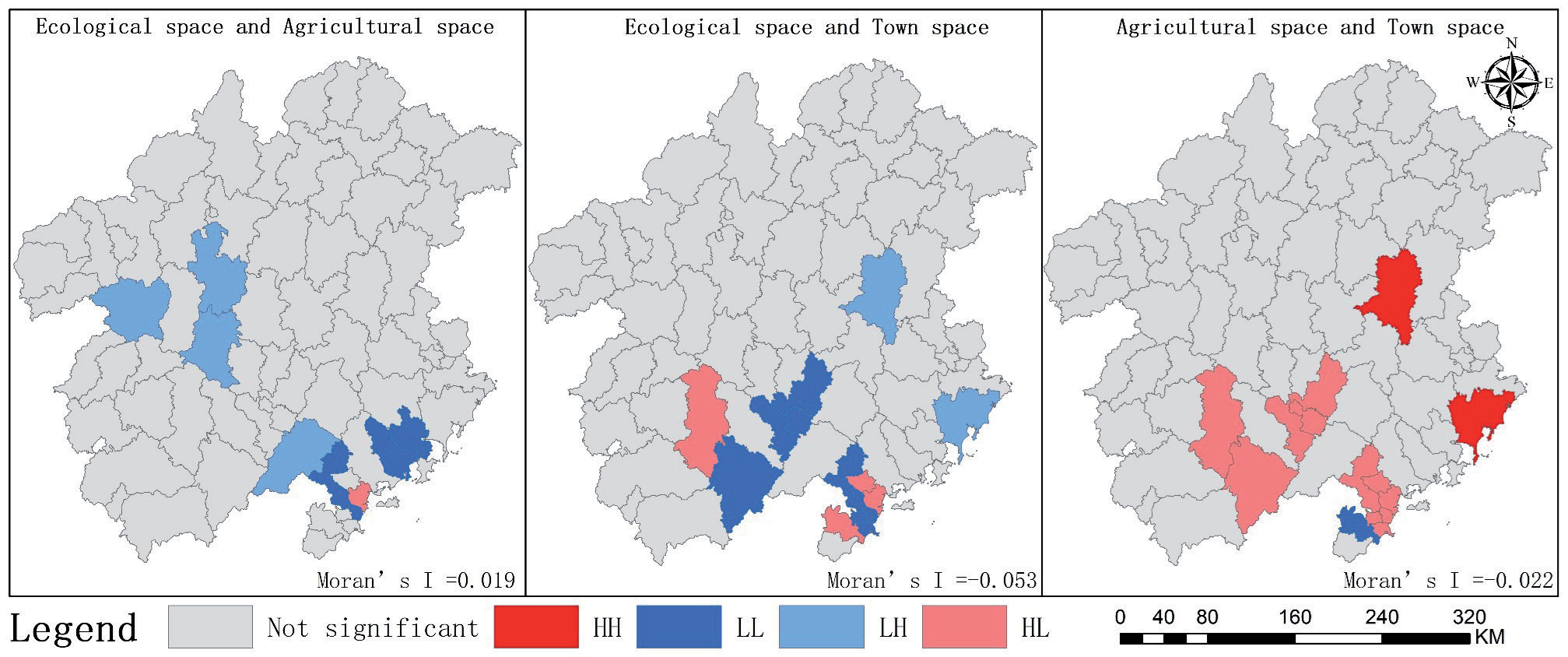
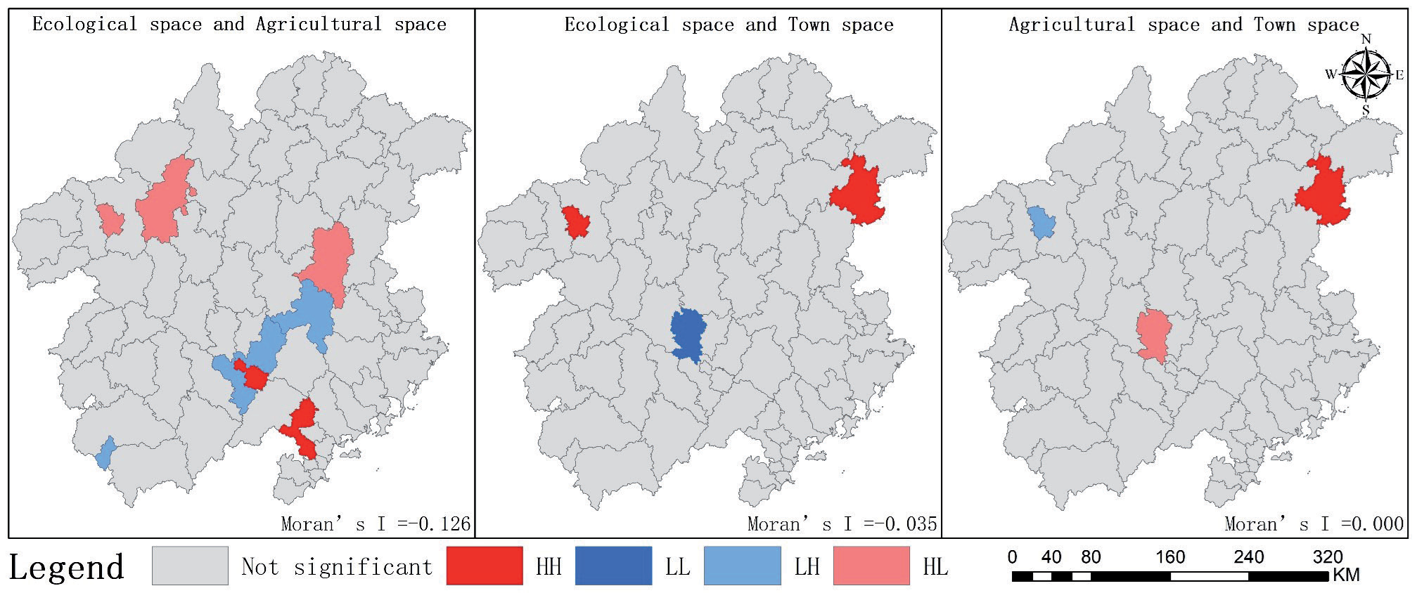
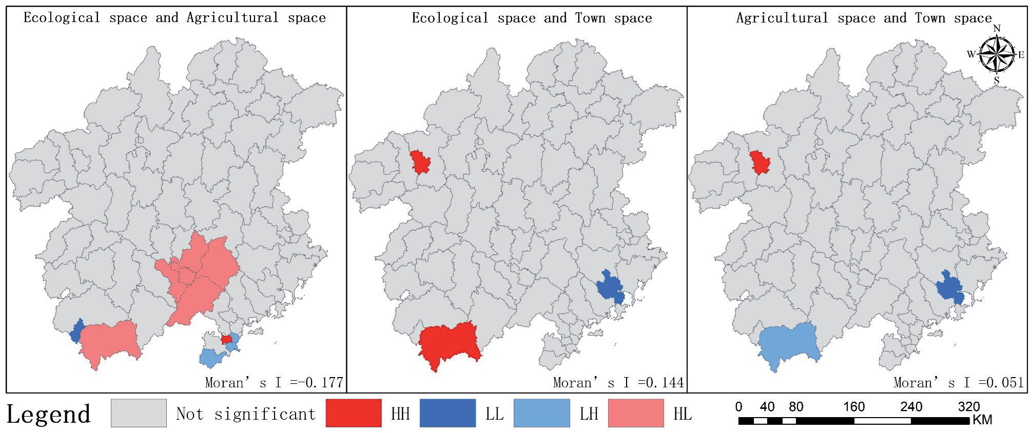
From the bivariate spatial correlation analysis (Table 4), most of the correlation coefficients are less than 0, indicating significant relationships between spatial changes across different territories, with the strongest correlations observed in the southern region. The correlation between changes in ecological space and agricultural space shifted from positive to negative, with the absolute value initially increasing, then decreasing, and ultimately increasing again. In the bivariate spatial autocorrelation analysis (Figs. 13–16), from 2000 to 2005, the relationship between these spaces fluctuated, with LL agglomeration predominantly located in Longhai District, Xiangcheng District, Zhangpu County, and Changtai District in the coastal area. From 2005 to 2010, the relationship continued to fluctuate, with LH agglomeration primarily in Meixian District and Yongding District. From 2015 to 2020, the relationship oscillated with HL agglomeration being dominant, situated in Meixian District, Meijiang District, Fenshun County, and Taipo County.
The correlation between changes in ecological space and urban space was negatively correlated, with the absolute value first decreasing, then increasing, and finally decreasing again. From 2000 to 2005, the relationship between these spaces fluctuated, with LH agglomeration primarily located in Changtai District, Zhangpu County, Xiangcheng District, and Nanjing County. From 2005 to 2010, the relationship continued to fluctuate, with LL agglomeration primarily found in Meizhou City and Shantou City. From 2010 to 2015, the relationship oscillated, with HL agglomeration being dominant, situated in Meizhou City and Shantou City. From 2015 to 2020, the relationship continued to fluctuate, with more dispersed agglomeration areas.
The correlation between changes in agricultural space and urban space was negatively correlated, with the absolute value first decreasing and then increasing. From 2000 to 2005, the relationship between these spaces fluctuated, with LH agglomeration primarily located in Zhangzhou City and Longyan City. From 2005 to 2010, the relationship continued to fluctuate, with HL agglomeration predominantly found in Meizhou City, Shantou City, and Chaozhou City. From 2010 to 2015, the relationship oscillated, with agglomeration areas becoming more dispersed. From 2015 to 2020, the pattern continued with dispersed agglomeration areas [36].
Analysis of Drivers of Territorial Spatial Evolution
Driver Analysis
The characteristics of territorial spatial changes are influenced by a variety of factors, including nature, economy, society, transportation, and policies. The driving forces and intensities of various types of territorial spatial changes also differ. Utilizing social and humanistic data from past years and applying the geodetector model, the drivers of three types of spatial changes within the national territory of the study area were analyzed (Tables 5-7).
Table 4.
Correlation coefficient of spatial variation in land.
In terms of ecological space, from 2000 to 2005, the top three drivers leading to ecological spatial changes were the rate of change in average annual temperature (0.964), total retail sales of consumer goods (0.962), and GDP per capita (0.932). An increase in total retail sales indicates a rise in consumption levels, which contributes to an increase in per capita GDP and promotes the rapid expansion of urban land. Changes in temperature lead to ecological instability, affecting the overall scale of ecological space. During the 2005-2010 period, the rate of change in fixed asset investment rose sharply (0.999), the rate of change in average annual rainfall remained high (0.999), and the rate of change in per capita GDP was also at the top (0.999). Increases in fixed asset investment and per capita GDP reflect rapid economic development and urban expansion, leading to an increase in urban territorial space. From 2010 to 2015, the rate of change in annual average temperature ranked first (0.961), followed by the rates of change in road freight volume and road passenger volume. The increase in total freight and passenger volume indicates rapid development in transportation, necessitating the construction of urban roads to support industrial development in the Pearl River Delta. The drivers of ecological and spatial changes from 2015 to 2020 included the rate of change in annual average temperature (0.999) and total fixed asset investment (0.999), with the change in the proportion of tertiary industry value added to GDP ranking third (0.997). The increase in fixed asset investment and tertiary industry value added, along with the implementation of the PRD industry, promotes the development of the tertiary sector. The arrival of industries in the Pearl River Delta not only brings economic vitality but also necessitates significant urban industrial land, leading to urban expansion that encroaches on a large amount of ecological space. The level of economic development is the dominant factor leading to changes in ecological space [37].
In terms of agricultural space, the top three driving factors leading to the spatial divergence in the rate of change of agricultural space from 2000 to 2005 were the rate of change in the proportion of value added of the tertiary industry in GDP (0.837), local government expenditure in the general budget (0.817), and the rate of change in average annual temperature (0.812). Both the proportion of the tertiary industry and financial expenditures showed positive increases, clearly indicating that the focus of the policy environment did not prioritize agricultural space. From 2005 to 2010, the top three drivers were the rate of change in average annual rainfall (0.983), investment in fixed assets (0.901), and per capita GDP (0.883). The rate of change in average annual rainfall, having risen from the bottom to the top, led to deteriorating farming conditions in some areas, which was associated with a decrease in agricultural space. Moreover, the increased investment in fixed assets not only accelerated urban development but also drew rural populations to cities, further reducing agricultural space. From 2010 to 2015, the leading factors were the rate of change in annual temperature (0.903), the total amount of freight transported by road (0.863), and the ratio of the tertiary industry (0.851). The rate of change in temperature and the decrease in rainfall, along with climate change, had significant impacts on the agro-ecological space. From 2015 to 2020, the top factors were the rate of change in the share of the tertiary industry (0.911), average annual rainfall (0.908), and investment in fixed assets (0.908). These changes were not significantly different from the previous period. The arrival of industries in the Pearl River Delta squeezed agricultural land space. However, the decrease in rainfall, climate changes, and the impact of agricultural protection policies slowed the reduction of agricultural land space [38].
Table 5.
Detection of driving factors of ecological spatial rate of change.
[i] Note: A-K denotes the rate of change of eleven driving factors: average annual precipitation, average annual temperature, road passenger traffic, road freight traffic, population density, retail sales of consumer goods, per capita GDP, value added of the tertiary industry as a share of GDP, science and technology expenditures, fixed-asset investment, and general budgetary expenditures of the local Treasury, respectively.
In terms of urban space, the top three drivers of the spatial evolution of cities and towns from 2000 to 2005 were the rate of change in science and technology expenditures (0.990), the total amount of consumer goods (0.974), and the proportion of the tertiary industry (0.951). Increases in science and technology expenditures, total consumer goods, and the proportion of the tertiary industry positively impacted the spatial evolution of cities and towns. From 2005 to 2010, the leading factors in urban spatial evolution were the rate of change in average annual temperature (0.912), total retail sales of consumer goods (0.894), and total volume of road freight (0.771). The growth in total retail sales and road freight volume reflects rapid economic development and a rise in population consumption levels. These increases not only fostered economic growth but also promoted the expansion of urban space. For the period from 2010 to 2015, the most significant changes were seen in average annual rainfall (0.936), total retail sales of consumer goods (0.960), and science and technology expenditures (0.859). These factors indicated that rapid economic development and increased social consumption continued to drive the spatial expansion of cities and towns. From 2015 to 2020, the primary drivers were the rate of change in road freight transportation (0.953), population density (0.854), and science and technology expenditures (0.848). A notable shift occurred with the rate of change in population density moving to second place, where a decrease in population density had a counteracting effect on urban space. Meanwhile, increases in road freight transportation and science and technology expenditures continued to drive urban expansion. The influx of industries into the Pearl River Delta accelerated economic development, boosted social consumption, and attracted science and technology investments, all contributing to urban space expansion. However, due to the rapid urban expansion in previous years, the focus of urbanization shifted from incremental expansion to the revitalization of existing urban areas [39].
Table 6.
Detection of driving factors for the rate of change in agriculture.
[i] Note: A-K denotes the rate of change of eleven driving factors: average annual precipitation, average annual temperature, road passenger traffic, road freight traffic, population density, retail sales of consumer goods, per capita GDP, value added of the tertiary industry as a share of GDP, science and technology expenditures, fixed-asset investment, and general budgetary expenditures of the local Treasury, respectively.
Table 7.
Detection of driving factors for the rate of change in urban space.
[i] Note: A-K denotes the rate of change of eleven driving factors: average annual precipitation, average annual temperature, road passenger traffic, road freight traffic, population density, retail sales of consumer goods, per capita GDP, value added of the tertiary industry as a share of GDP, science and technology expenditures, fixed-asset investment, and general budgetary expenditures of the local Treasury, respectively.
Analysis of Driving Mechanisms
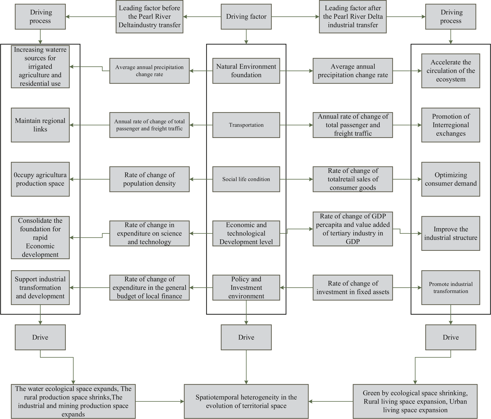
Based on the variations in influencing factors of land space change across different periods within the study area, the top three driving factors were selected for each period, and a systematic analysis was conducted to elucidate the driving mechanisms of land space change in the Hanjiang River Basin after the implementation of industrial transfers from the Pearl River Delta (Fig. 17).
(1) Before the industrial transfer from the Pearl River Delta, the economy of the Hanjiang River Basin lacked foundational industries, which necessitated reliance on large-scale land development and intense utilization. This led to the formation of a territorial spatial pattern predominantly characterized by tourism and agriculture. On one hand, much of the Hanjiang River Basin consists of hilly terrain, unsuitable for agricultural cultivation. This, coupled with abundant rainfall, frequently resulted in flooding. Consequently, there was a modest increase in water ecological space and a reduction in the area available for agricultural production, compressing the agricultural land space. On the other hand, the absence of sufficient industrial employment opportunities triggered a significant migration of the rural population to urban areas. Cities began to expand their urban spaces to accommodate this labor influx, further compressing ecological national space [40].
(2) Post-transfer, the Hanjiang River Basin benefited from its natural geographical proximity to the PRD region and its administrative alignment within Guangdong Province, similar to the PRD. This facilitated the reception of some industries from the PRD, which significantly altered the spatial pattern of the national territory. On one hand, a decrease in rainfall and increased water supply pressure led to a slight reduction in water territorial space. On the other hand, the region's adoption of certain industries from the Pearl River Delta, many of which are heavily polluting, necessitated a trade-off between ecological space and economic development. Investments in fixed assets from earlier periods laid the groundwork for this industrial takeover, causing a shift in township construction from incremental expansion to revitalization of existing stocks. This transition slowed the growth of towns and cities. Moreover, the reduction in rainfall and flooding further decelerated the decrease in agricultural land space. With the acquisition of industries from the Pearl River Delta, the Hanjiang River Basin gradually enhanced its industrial structure through significant capital investments and increased capacity for innovation.
Conclusion and Outlook
This study analyzes the evolution of land space in economically developed watersheds based on the logical framework of "evolution process - evolution pattern - driving force." This analysis aims to provide useful references for the rational and orderly development and protection patterns of land use, leading to the following key conclusions:
(1) Temporal changes from 2000 to 2020: The land space in the study area primarily comprised ecological spaces, with variations in the evolution of land space types across different periods. Urban living spaces and industrial and mining production spaces exhibited increasing trends. Rural living space initially increased and then decreased, while rural production space consistently decreased. Water ecological space and green cover ecological space both followed a pattern of initial increase followed by a decrease. Overall, agricultural and ecological spaces have been gradually diminishing, whereas urban space has been expanding and evolving. Ecological and agricultural spaces frequently transformed into each other, with agricultural space also showing interchangeability. The expansion of urban space predominantly encroached upon ecological and agricultural spaces.
(2) Spatial pattern evolution: The evolution of the land space pattern in the study area demonstrated regular changes. The center of gravity of urban space shifted from southwest to northeast, then from southeast to northwest [41]. Ecological space's center of gravity initially moved from northwest to southeast, then meandered in the opposite direction, surpassing its 2000 starting point. Agricultural space's center of gravity shifted from southwest to northeast and then converged back to the starting point from northeast to southwest. Town space exhibited univariate high and high agglomeration characteristics centrally, while low and low agglomeration shifted southward. Agricultural space showed a central high and high agglomeration. The spatial distribution of ecological space was more dispersed. The bivariate administrative unit of high and low agglomeration of agricultural space in town space shifted from north to south, and the spatial distributions of ecological space in town space and agricultural space were more decentralized.
(3) Driving factors: Average annual precipitation and fixed asset investment were the primary factors influencing the evolution of ecological space. The significant impact on agricultural space was determined by the proportion of tertiary industry value-added in GDP and average annual precipitation [33]. Total retail sales of consumer goods were the predominant drivers of urban space evolution.
This study extends and enhances the empirical research on land use/cover change, revealing the development processes, spatial patterns, and driving factors of the spatial and temporal evolution of the land space in the Han River Basin. It provides valuable insights for optimizing land space patterns. Compared to inland areas, the Han River Basin is economically advanced but exhibits more pronounced land space changes and a more fragile ecosystem. The frequent conversions of land space can destabilize regional development, which is detrimental to long-term sustainable growth. Therefore, conducting a "dual evaluation" of the river basin, drafting specialized plans for land space management, and clarifying the carrying capacity and suitability levels for regional development are crucial research focuses and directions for establishing a rational and orderly pattern of land space protection and development.

